8. Learning as conditional inference
The line between “reasoning” and “learning” is unclear in cognition. Just as reasoning can be seen as a form of conditional inference, so can learning: discovering persistent facts about the world (for example, causal processes or causal properties of objects). By saying that we are learning “persistent” facts we are indicating that there is something to infer which we expect to be relevant to many observations over time. Thus, we will formulate learning as inference in a model that (1) has a fixed latent value of interest, the hypothesis, and (2) has a sequence of observations, the data points. This will be a special class of models for sequences of observations—those that fit the pattern of Bayes rule:
(query
 (define hypothesis (prior))
 hypothesis
 (equal? observed-data (repeat N (lambda () (observe hypothesis)))))
The prior samples a hypothesis from the hypothesis space. This function expresses our prior knowledge about how the process we observe is likely to work, before we have observed any data. The observe function describes how a data point is generated given the hypothesis. What can be inferred about the hypothesis given a certain subset of the observed data? How much more can we learn as the size of the observed data set increases—what is the learning curve?
Example: Learning About Coins
As a simple illustration of learning, imagine that a friend pulls a coin out of her pocket and offers it to you to flip. You flip it five times and observe a set of all heads:
(H H H H H).
Does this seem at all surprising? To most people, flipping five heads in a row is a minor coincidence but nothing to get excited about. But suppose you flip it five more times and continue to observe only heads. Now the data set looks like this:
(H H H H H H H H H H).
Most people would find this a highly suspicious coincidence and begin to suspect that perhaps their friend has rigged this coin in some way – maybe it’s a weighted coin that always comes up heads no matter how you flip it. This inference could be stronger or weaker, of course, depending on what you believe about your friend or how she seems to act; did she offer a large bet that you would flip more heads than tails? Now you continue to flip five more times and again observe nothing but heads – so the data set now consists of 15 heads in a row:
(H H H H H H H H H H H H H H H).
Regardless of your prior beliefs, it is almost impossible to resist the inference that the coin is a trick coin.
This “learning curve” reflects a highly systematic and rational process of conditional inference. For simplicity let’s consider only two hypotheses, two possible definitions of coin, representing a fair coin and a trick coin that produces heads 95% of the time. A priori, how likely is any coin offered up by a friend to be a trick coin? Of course there is no objective or universal answer to that question, but for the sake of illustration let’s assume that the prior probability of seeing a trick coin is 1 in a 1000, versus 999 in 1000 for a fair coin. These probabilities determine the weight passed to make-coin. Now to inference:
(define observed-data '(h h h h h))
(define num-flips (length observed-data))

(define samples
  (mh-query
     1000 10

     (define fair-prior 0.999)
     (define fair-coin? (flip fair-prior))

     (define make-coin (lambda (weight) (lambda () (if (flip weight) 'h 't))))
     (define coin (make-coin (if fair-coin? 0.5 0.95)))

     fair-coin?

     (equal? observed-data (repeat num-flips coin))))

(hist samples "Fair coin?")
Try varying the number of flips and the number of heads observed. You should be able to reproduce the intuitive learning curve described above. Observing 5 heads in a row is not enough to suggest a trick coin, although it does raise the hint of this possibility: its chances are now a few percent, approximately 30 times the baseline chance of 1 in a 1000. After observing 10 heads in a row, the odds of trick coin and fair coin are now roughly comparable, although fair coin is still a little more likely. After seeing 15 or more heads in a row without any tails, the odds are now strongly in favor of the trick coin.
Study how this learning curve depends on the choice of fair-prior. There is certainly a dependence. If we set fair-prior to be 0.5, equal for the two alternative hypotheses, just 5 heads in a row are sufficient to favor the trick coin by a large margin. If fair-prior is 99 in 100, 10 heads in a row are sufficient. We have to increase fair-prior quite a lot, however, before 15 heads in a row is no longer sufficient evidence for a trick coin: even at fair-prior = 0.9999, 15 heads without a single tail still weighs in favor of the trick coin. This is because the evidence in favor of a trick coin accumulates exponentially as the data set increases in size; each successive H flip increases the evidence by nearly a factor of 2.
Learning is always about the shift from one state of knowledge to another. The speed of that shift provides a way to diagnose the strength of a learner’s initial beliefs. Here, the fact that somewhere between 10 and 15 heads in a row is sufficient to convince most people that the coin is a trick coin suggests that for most people, the a priori probability of encountering a trick coin in this situation is somewhere between 1 in a 100 and 1 in 10,000—a reasonable range. Of course, if you begin with the suspicion that any friend who offers you a coin to flip is liable to have a trick coin in his pocket, then just seeing five heads in a row should already make you very suspicious—as we can see by setting fair-prior to a value such as 0.9.
Learning a Continuous Parameter
The previous example represents perhaps the simplest imaginable case of learning. Typical learning problems in human cognition or AI are more complex in many ways. For one, learners are almost always confronted with more than two hypotheses about the causal structure that might underlie their observations. Indeed, hypothesis spaces for learning are often infinite. Countably infinite hypothesis spaces are encountered in models of learning for domains traditionally considered to depend on “discrete” or “symbolic” knowledge; hypothesis spaces of grammars in language acquisition are a canonical example. Hypothesis spaces for learning in domains traditionally considered more “continuous”, such as perception or motor control, are typically uncountable and parametrized by one or more continuous dimensions. In causal learning, both discrete and continuous hypothesis spaces typically arise. In statistics and machine learning, making conditional inferences over continuous hypothesis spaces given data is usually called parameter estimation.
We can explore a basic case of learning with continuous hypothesis spaces by slightly enriching our coin flipping example. Suppose that our hypothesis generator make-coin, instead of simply flipping a coin to determine which of two coin weights to use, can choose any coin weight between 0 and 1.
The following program computes conditional inferences about the weight of a coin drawn from a prior distribution described by the uniform function, conditioned on a set of observed flips.
(define observed-data '(h h h h h))
(define num-flips (length observed-data))
(define num-samples 1000)
(define prior-samples (repeat num-samples (lambda () (uniform 0 1))))

(define samples
  (mh-query
   num-samples 10

   (define coin-weight (uniform 0 1))

   (define make-coin (lambda (weight) (lambda () (if (flip weight) 'h 't))))
   (define coin (make-coin coin-weight))

   coin-weight

   (equal? observed-data (repeat num-flips coin))))

(density prior-samples "Coin weight, prior to observing data")
(density samples "Coin weight, conditioned on observed data")
Because the output of inference is a set of conditional samples, and each sample is drawn from the uncountable interval \([0,1]\), we cannot expect that any of these samples will correspond exactly to the true coin weight or the single most likely value.
Experiment with different data sets, varying both the number of flips and the relative proportion of heads and tails. How does the shape of the conditional distribution change? The location of its peak reflects a reasonable “best guess” about the underlying coin weight. It will be roughly equal to the proportion of heads observed, reflecting the fact that our prior knowledge is basically uninformative; a priori, any value of coin-weight is equally likely. The spread of the conditional distribution reflects a notion of confidence in our beliefs about the coin weight. The distribution becomes more sharply peaked as we observe more data, because each flip, as an independent sample of the process we are learning about, provides additional evidence the process’s unknown parameters.
When studying learning as conditional inference, that is when considering an ideal learner model, we are particularly interested in the dynamics of how inferred hypotheses change as a function of amount of data (often thought of as time the learner spends acquiring data). We can map out the trajectory of learning by plotting a summary of the posterior distribution over hypotheses as a function of the amount of observed data. Here we plot the mean of the samples of the coin weight (the expected weight) in the above example:
(define make-coin (lambda (weight) (lambda () (if (flip weight) 'h 't))))

(define (samples data)
  (mh-query
   400 10

   (define coin-weight (uniform 0 1))

   (define coin (make-coin coin-weight))

   coin-weight

   ;; use factor statement to simulate flipping the coin and obtaining each observation
   (factor (sum (map
                 (lambda (obs) (if (equal? obs 'h)
                                   (log coin-weight)
                                   (log (- 1 coin-weight))))

                 data)))))

(define true-weight 0.9)
(define true-coin (make-coin true-weight))
(define full-data-set (repeat 100 true-coin))
(define observed-data-sizes '(1 3 6 10 20 30 50 70 100))
(define (estimate N) (mean (samples (take full-data-set N))))
(lineplot (map (lambda (N) (list N (estimate N)))
               observed-data-sizes))
Try plotting different kinds of statistics, e.g., the absolute difference between the true mean and the estimated mean (using the function abs), or a confidence measure like the standard error of the mean.
Notice that different runs of this program can give quite different trajectories, but always end up in the same place in the long run. This is because the data set used for learning is different on each run. Of course, we are often interested in the average behavior of an ideal learner: we would average this plot over many randomly chosen data sets, simulating many different learners (however, this is too time consuming for a quick simulation).
What if we would like to learn about the weight of a coin, or any parameters of a causal model, for which we have some informative prior knowledge? It is easy to see that the previous Church program doesn’t really capture our prior knowledge about coins, or at least not in the most familiar everyday scenarios. Imagine that you have just received a quarter in change from a store – or even better, taken it from a nicely wrapped-up roll of quarters that you have just picked up from a bank. Your prior expectation at this point is that the coin is almost surely fair. If you flip it 10 times and get 7 heads out of 10, you’ll think nothing of it; that could easily happen with a fair coin and there is no reason to suspect the weight of this particular coin is anything other than 0.5. But running the above query with uniform prior beliefs on the coin weight, you’ll guess the weight in this case is around 0.7. Our hypothesis generating function needs to be able to draw coin-weight not from a uniform distribution, but from some other function that can encode various expectations about how likely the coin is to be fair, skewed towards heads or tails, and so on. We use the beta distribution:
(define observed-data '(h h h t h t h h t h))
(define num-flips (length observed-data))
(define num-samples 1000)
(define pseudo-counts '(10 10))
(define prior-samples (repeat num-samples (lambda () (beta (first pseudo-counts)
                                                           (second pseudo-counts)))))

(define samples
  (mh-query
   num-samples 10

   (define coin-weight (beta (first pseudo-counts) (second pseudo-counts)))

   (define make-coin (lambda (weight) (lambda () (if (flip weight) 'h 't))))
   (define coin (make-coin coin-weight))

   coin-weight

   (equal? observed-data (repeat num-flips coin))))

(density prior-samples "Coin weight, prior to observing data")
(density samples "Coin weight, conditioned on observed data")
Is the family of Beta distributions sufficient to represent all of people’s intuitive prior knowledge about the weights of typical coins? It would be mathematically appealing if so, but unfortunately people’s intuitions are too rich to be summed up with a single Beta distribution. To see why, imagine that you flip this quarter fresh from the bank and flip it 25 times, getting heads every single time! Using a Beta prior with pseudo-counts of 100, 100 or 1000, 1000 seems reasonable to explain why seeing 7 out of 10 heads does not move our conditional estimate of the weight very much at all from its prior value of 0.5, but this doesn’t fit at all what we think if we see 25 heads in a row. Try running the program above with a coin weight drawn from \(\text{Beta}(100,100)\) and an observed data set of 25 heads and no tails. The most likely coin weight in the conditional inference now shifts slightly towards a heads-bias, but it is far from what you would actually think given these (rather surprising!) data. No matter how strong your initial belief that the bank roll was filled with fair coins, you’d think: “25 heads in a row without a single tail? Not a chance this is a fair coin. Something fishy is going on… This coin is almost surely going to come up heads forever!” As unlikely as it is that someone at the bank has accidentally or deliberately put a trick coin in your fresh roll of quarters, that is not nearly as unlikely as flipping a fair coin 25 times and getting no tails.
Imagine the learning curve as you flip this coin from the bank and get 5 heads in a row… then 10 heads in a row… then 15 heads… and so on. Your beliefs seem to shift from “fair coin” to “trick coin” hypotheses discretely, rather than going through a graded sequence of hypotheses about a continuous coin weight moving smoothly between 0.5 and 1. It is clear that this “trick coin” hypothesis, however, is not merely the hypothesis of a coin that always (or almost always) comes up heads, as in the first simple example in this section where we compared two coins with weight 0.5 and 0.95. Suppose that you flipped a quarter fresh from the bank 100 times and got 85 heads and 15 tails. As strong as your prior belief starts out in favor of a fair coin, this coin also won’t seem fair. Using a strong beta prior (e.g., \(\text{Beta}(100,100)\) or \(\text{Beta}(1000,1000)\)) suggests counterintuitively that the weight is still near 0.5 (respectively, 0.52 or 0.62). Given the choice between a coin of weight 0.5 and 0.95, weight 0.95 is somewhat more likely. But neither of those choices matches intuition at this point, which is probably close to the empirically observed frequency: “This coin obviously isn’t fair, and given that it came up heads 85/100 times, my best guess is it that it will come heads around 85% of the time in the future.” Confronted with these anomalous sequences, 25/25 heads or 85/100 heads from a freshly unwrapped quarter, it seems that the evidence shifts us from an initially strong belief in a fair coin (something like a \(\text{Beta}(1000,1000)\) prior) to a strong belief in a discretely different alternative hypothesis, a biased coin of some unknown weight (more like a uniform or \(\text{Beta}(1,1)\) distribution). Once we make the transition to the biased coin hypothesis we can estimate the coin’s weight on mostly empirical grounds, effectively as if we are inferring that we should “switch” our prior on the coin’s weight from a strongly symmetric beta to a much more uniform distribution.
We will see later on how to explain this kind of belief trajectory – and we will see a number of learning, perception and reasoning phenomena that have this character. The key will be to describe people’s prior beliefs using more expressive programs than we can capture with a single XRP representing distributions familiar in statistics. Most real world problems of parameter estimation, or learning continuous parameters of causal models, are significantly more complex than this simple example. They typically involve joint inference over more than one parameter at a time, with a more complex structure of functional dependencies. They also often draw on stronger and more interestingly structured prior knowledge about the parameters, rather than just assuming uniform or beta initial beliefs. Our intuitive theories of the world have a more abstract structure, embodying a hierarchy of more or less complex mental models. Yet the same basic logic of how to approach learning as conditional inference applies.
Example: Estimating Causal Power
A common problem for cognition is causal learning: from observed evidence about the co-occurance of events, attempt to infer the causal structure relating them. An especially simple case that has been studied by psychologists is elemental causal induction: causal learning when there are only two events, a potential cause C and a potential effect E. Cheng and colleagues [@Cheng] have suggested assuming that C and background effects can both cause C, with a noisy-or interaction. Causal learning then because an example of parameter learning, where the parameter is the “causal power” of C to cause E:
(define samples
  (mh-query 10000 1
            (define cp (uniform 0 1)) ;;causal power of C to cause E.
            (define b (uniform 0 1))  ;;background probability of E.

            ;;the noisy causal relation to get E given C:
            (define (E-if-C C)
              (or (and C (flip cp))
                  (flip b)))

            ;;infer the causal power:
            cp

            ;;condition on some contingency evidence:
            (and (E-if-C true)
                 (E-if-C true)
                 (not (E-if-C false))
                 (E-if-C true))))

(hist samples)
Experiment with this model: when does it conclude that a causal relation is likely (high cp)? Does this match your intuitions? What role does the background rate b play? What happens if you change the functional relationship in E-if-C?
Grammar-based Concept Induction
An important worry about Bayesian models of learning is that the Hypothesis space must either be too simple, as in the models above, specified in a rather ad-hoc way, or both. There is a tension here: human representations of the world are enormously complex and so the space of possible representations must be correspondingly big, and yet we would like to understand the representational resources in simple and uniform terms. How can we construct very large (possibly infinite) hypothesis spaces, and priors over them, with limited tools? One possibility is to use a grammar to specify a hypothesis language: a small grammar can generate an infinite array of potential hypotheses. Because grammars are themselves generative processes, a prior is provided as well.
Example: Inferring an Arithmetic Expression
Consider the following Church program, which induces an arithmetic function from examples. We generate an expression as a list, and then turn it into a value (in this case a procedure) by using eval—a function that invokes evaluation.
(define (random-arithmetic-expression)
  (if (flip 0.7)
      (if (flip) 'x (sample-integer 10))
      (list (uniform-draw '(+ -)) (random-arithmetic-expression) (random-arithmetic-expression))))

(define (procedure-from-expression expr)
  (eval (list 'lambda '(x) expr)))

(define (sample)
(rejection-query

 (define my-expr (random-arithmetic-expression))
 (define my-proc (procedure-from-expression my-expr))

 my-expr

 (= (my-proc 1) 3)))

(apply display (repeat 20 sample))
The query asks for an arithmetic expression on variable x such that it evaluates to 3 when x is 1. In this example there are many extensionally equivalent ways to satisfy the condition, for instance the expressions 3, (+ 1 2), and (+ x 2), but because the more complex expressions require more choices to generate, they are chosen less often. What happens if we observe more data? For instance, try changing the condition in the above query to (and (= (my-proc 1) 3) (= (my-proc 2) 4)). Using eval can be rather slow, so here’s another formulation that directly builds the arithmetic function by random combination of subfunctions:
(define (random-arithmetic-fn)
  (if (flip 0.3)
      (random-combination (random-arithmetic-fn) (random-arithmetic-fn))
      (if (flip)
          (lambda (x) x)
          (random-constant-fn))))

(define (random-combination f g)
  (define op (uniform-draw (list + -)))
  (lambda (x) (op (f x) (g x))))

(define (random-constant-fn)
  (define i (sample-integer 10))
  (lambda (x) i))


(define (sample)
  (rejection-query

   (define my-proc (random-arithmetic-fn))

   (my-proc 2)

   (= (my-proc 1) 3)))

(repeat 100 sample)

(hist (repeat 500 sample))
This model learns from an infinite hypothesis space—all expressions made from ‘x’, ‘+’, ‘-’, and constant integers—but specifies both the hypothesis space and its prior using the simple generative process random-arithmetic-expression.
Example: Rational Rules
How can we account for the productivity of human concepts (the fact that every child learns a remarkable number of different, complex concepts)? The “classical” theory of concepts formation accounted for this productivity by hypothesizing that concepts are represented compositionally, by logical combination of the features of objects (see for example Bruner, Goodnow, and Austin, 1951). That is, concepts could be thought of as rules for classifying objects (in or out of the concept) and concept learning was a process of deducing the correct rule.
While this theory was appealing for many reasons, it failed to account for a variety of categorization experiments. Here are the training examples, and one transfer example, from the classic experiment of Medin and Schaffer (1978). The bar graph above the stimuli shows the portion of human participants who said that bug was a “fep” in the test phase (the data comes from a replication by Nosofsky, Gluck, Palmeri, McKinley (1994); the bug stimuli are courtesy of Pat Shafto):
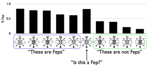
Notice three effects: there is a gradient of generalization (rather than all-or-nothing classification), some of the Feps are better (or more typical) than others (this is called “typicality”), and the transfer item is a ‘’better’’ Fep than any of the Fep exemplars (this is called “prototype enhancement”). Effects like these were difficult to capture with classical rule-based models of category learning, which led to deterministic behavior. As a result of such difficulties, psychological models of category learning turned to more uncertain, prototype and exemplar based theories of concept representation. These models were able to predict behavioral data very well, but lacked compositional conceptual structure.
Is it possible to get graded effects from rule-based concepts? Perhaps these effects are driven by uncertainty in learning rather than uncertainty in the representations themselves? To explore these questions Goodman, Tenenbaum, Feldman, and Griffiths (2008) introduced the Rational Rules model, which learns deterministic rules by probabilistic inference. This model has an infinite hypothesis space of rules (represented in propositional logic), which are generated compositionally. Here is a slightly simplified version of the model, applied to the above experiment:
;;first set up the training (cat A/B) and test objects:
(define num-features 4)

(define A-objects (list '(0 0 0 1) '(0 1 0 1) '(0 1 0 0) '(0 0 1 0) '(1 0 0 0)))

(define B-objects (list '(0 0 1 1) '(1 0 0 1) '(1 1 1 0) '(1 1 1 1)))

(define T-objects (list '(0 1 1 0) '(0 1 1 1) '(0 0 0 0) '(1 1 0 1)
                        '(1 0 1 0) '(1 1 0 0) '(1 0 1 1)))

;;here are the human results from Nosofsky et al, for comparison:
(define human-A '(0.77 0.78 0.83 0.64 0.61))
(define human-B '(0.39 0.41 0.21 0.15))
(define human-T '(0.56 0.41 0.82 0.40 0.32 0.53 0.20))

;;two parameters: stopping probability of the grammar, and noise probability:
(define tau 0.3)
(define noise-param (exp -1.5))

;;a generative process for disjunctive normal form propositional equations:
(define (get-formula)
  (if (flip tau)
      (let ((c (Conj))
            (f (get-formula)))
        (lambda (x) (or (c x) (f x))))
      (Conj)))

(define (Conj)
  (if (flip tau)
      (let ((c (Conj))
            (p (Pred)))
        (lambda (x) (and (c x) (p x))))
      (Pred)))

(define (Pred)
  (let ((index (sample-integer num-features))
        (value (sample-integer 2)))
    (lambda (x) (= (list-ref x index) value))))


(define (noisy-equal? a b) (flip (if (equal? a b) 0.999999999 noise-param)))

(define samples
  (mh-query
   1000 10

   ;;infer a classification formula
   (define my-formula (get-formula))

   ;;look at posterior predictive classification
   (map my-formula (append T-objects A-objects B-objects))

   ;;conditioning (noisily) on all the training eamples:
   (and (all (map (lambda (x) (noisy-equal? true (my-formula x))) A-objects))
        (all (map (lambda (x) (noisy-equal? false (my-formula x))) B-objects)))))


;;now plot the predictions vs human data:
(define (means samples)
  (if (null? (first samples))
      '()
      (pair (mean (map (lambda (x) (if x 1.0 0.0)) (map first samples)))
            (means (map rest samples)))))

(scatter (map pair (means samples) (append human-T human-A human-B)) "model vs human")
Goodman, et al, have used to this model to capture a variety of classic categorization effects (Goodman, Tenenbaum, Feldman, & Griffiths, 2008). Thus probabilistic induction of (deterministic) rules can capture many of the graded effects previously taken as evidence against rule-based models.
This style of compositional concept induction model, can be naturally extended to more complex hypothesis spaces. For examples, see:
Compositionality in rational analysis: Grammar-based induction for concept learning. N. D. Goodman, J. B. Tenenbaum, T. L. Griffiths, and J. Feldman (2008). In M. Oaksford and N. Chater (Eds.). The probabilistic mind: Prospects for Bayesian cognitive science.
A Bayesian Model of the Acquisition of Compositional Semantics. S. T. Piantadosi, N. D. Goodman, B. A. Ellis, and J. B. Tenenbaum (2008). Proceedings of the Thirtieth Annual Conference of the Cognitive Science Society.
It has been used to model theory acquisition, learning natural numbers concepts, etc. Further, there is no reason that the concepts need to be deterministic; in Church stochastic functions can be constructed compositionally and learned by induction:
- Learning Structured Generative Concepts. A. Stuhlmueller, J. B. Tenenbaum, and N. D. Goodman (2010). Proceedings of the Thirty-Second Annual Conference of the Cognitive Science Society.
References
Goodman:2008p865Goodman, N. D., Tenenbaum, J. B., Feldman, J., & Griffiths, T. L. (2008). A rational analysis of rule-based concept learning. Cognitive Science.