12. Non-parametric models

By: Noah Goodman, Timothy J. O’Donnell, Josh Tenenbaum

In the chapter on Mixture Models we saw a simple way to construct a model with an unbounded number of categories—simply place uncertainty over the number of categories that are ‘actually’ in the world. In this section we describe another approach which instead posits an infinite number of (mostly unused) categories actually in the world. The non-parametric, or infinite, models have a number of useful mathematical properties.

Prelude: sampling from a discrete distribution

In Church the discrete distribution is a primitive—you can simply call (sample-discrete '(0.2 0.3 0.1 0.4)). If it wasn’t built-in and the only random primitive you could use was flip, how could you sample from discrete? One solution is to recursively walk down the list of probabilities, deciding whether to stop on each step. For instance, in (sample-discrete '(0.2 0.3 0.1 0.4)) there is a 0.2 probability of stopping on the first flip, a 0.3/0.8 probability of stopping on the second flip (given that we didn’t stop on the first), and so on. We can start by turning the list of probabilities into a list of residual probabilities—the probability we will stop on each step, given that we haven’t stopped yet:

(define (residuals probs)
  (if (null? probs)
      '()
      (pair (/ (first probs) (sum probs))
            (residuals (rest probs)))))

(residuals '(0.2 0.3 0.1 0.4))

Now to sample from the discrete distribution we simply walk down this list, deciding when to stop:

(define (residuals probs)
  (if (null? probs)
      '()
      (pair (/ (first probs) (sum probs))
            (residuals (rest probs)))))

(define (my-sample-discrete resid)
  (if (null? resid)
      '()
      (if (flip (first resid))
          1
          (+ 1 (my-sample-discrete (rest resid))))))

(hist (repeat 5000 (lambda () (my-sample-discrete (residuals '(0.2 0.3 0.1 0.4))))) "stop?" )

Infinite Discrete Distributions: The Dirichlet Processes

We have seen several examples of mixture models where the mixture components are chosen from a multinomial distribution and the weights of the mixture components are drawn from a Dirichlet prior. Both multinomial and Dirichlet distributions are defined for fixed numbers of categories—now, imagine generalizing the combination of Dirichlet and multinomial, to a multinomial over infinitely many categories of components. This would solve the problem of “running out of categories,” because there would always be more categories that hadn’t yet been used for any observation.

Just as the Dirchlet distribution defines a prior on parameters for a multinomial with \(K\) possible outcomes, the Dirichlet process defines a prior on parameters for a multinomial with \(K = \infty\)—an infinite number of possible outcomes.

First, we imagine drawing an infinite sequence of samples from a beta distribution with parameters \(1,\ \alpha\) (recall that a beta distribution defines a distribution on the interval \([0,1]\)). We write this infinite set of draws as \(\left\{\beta'_k\right\}_{k=1}^{\infty}\). \[\beta'_k \sim \text{Beta}\left(1,\alpha\right)\] Ultimately we would like to define a distribution on an infinite set of discrete outcomes that will represent our categories or mixture components, but we start by defining a distribution on the natural numbers. The probability of the natural number \(k\) is given by: \[\beta_k = \prod_{i=1}^{k-1}\left(1-\beta'_i\right)\cdot\beta'_k\] How can this be interpreted as a generative process? Imagine “walking” down the natural numbers in order, flipping a coin with weight \(\beta'_i\) for each one; if the coin comes up false, we continue to the next natural number; if the coin comes up true, we stop and return the current natural number. Convince yourself that the probability of getting natural number \(k\) is given by \(\beta_k\) above.

To formalize this as a Church program, we define a procedure, pick-a-stick, that walks down the list of \(\beta'_k\)s (called sticks in the statistics and machine learning literatures) and flips a coin at each one: if the coin comes up true, it returns the index associated with that stick, if the coin comes up false the procedure recurses to the next natural number.

(define (pick-a-stick sticks J)
  (if (flip (sticks J))
      J
      (pick-a-stick sticks (+ J 1))))

(define sticks
 (mem (lambda (index) (beta 1 alpha))))

pick-a-stick is a higher-order procedure that takes another procedure called sticks, which returns the stick weight for each stick. pick-a-stick is also a recursive function—one that calls itself.

Notice that sticks uses mem to associate a particular draw from beta with each natural number. When we call it again with the same index we will get back the same stick weight. This (crucially) means that we construct the \(\beta'_k\)s only “lazily” when we need them—even though we started by imagining an infinite set of “sticks” we only ever construct a finite subset of them.

We can put these ideas together in a procedure called make-sticks which takes the \(\alpha\) parameter as an input and returns a procedure which samples stick indices.

(define (pick-a-stick sticks J)
  (if (flip (sticks J))
      J
      (pick-a-stick sticks (+ J 1))))

(define (make-sticks alpha)
  (let ((sticks (mem (lambda (x) (beta 1.0 alpha)))))
    (lambda () (pick-a-stick sticks 1))))

(define my-sticks (make-sticks 1))

(hist (repeat 1000 my-sticks) "Dirichlet Process")

my-sticks samples from the natural numbers by walking down the list starting at 1 and flipping a coin weighted by a fixed \(\beta'_k\) for each \(k\). When the coin comes up true it returns \(k\) otherwise it keeps going. It does this by drawing the individual \(\beta'_k\) lazily, only generating new ones when we have walked out further than furthest previous time. This way of constructing a Dirichlet Process is known as the stick-breaking construction and was first defined in:
Sethuraman, J. (1994). A constructive definition of dirichlet priors. Statistica Sinica, 4(2):639–650.
There are many other ways of defining a Dirichlet Process, one of which—the Chinese Restaurant Process—we will see below.

Stochastic Memoization with DPmem

The above construction of the Dirichlet process defines a distribution over the infinite set of natural numbers. We quite often want a distribution not over the natural numbers themselves, but over an infinite set of samples from some other distribution (called the base distribution): we can generalize the Dirichlet process to this setting by using mem to associate to each natural number a draw from the base distribution.

(define (pick-a-stick sticks J)
  (if (flip (sticks J))
      J
      (pick-a-stick sticks (+ J 1))))

(define (make-sticks alpha)
  (let ((sticks (mem (lambda (x) (beta 1.0 alpha)))))
    (lambda () (pick-a-stick sticks 1))))

(define (DPthunk alpha base-dist)
  (let ((augmented-proc (mem (lambda (stick-index) (base-dist))))
        (DP (make-sticks alpha)))
    (lambda () (augmented-proc (DP)))))


(define memoized-gaussian (DPthunk 1.0 (lambda () (gaussian 0.0 1.0))))
(density (repeat 10000 (lambda () (gaussian 0.0 1.0))) "Base Distribution" true)
(density (repeat 10000 memoized-gaussian) "Dirichlet Process" true)

We can do a similar transformation to any church procedure: we associate to every argument and natural number pair a sample from the procedure, then use the Dirichlet process to define a new procedure with the same signature. In Church this useful higher-order distribution is called DPmem:

(define (pick-a-stick sticks J)
  (if (flip (sticks J))
      J
      (pick-a-stick sticks (+ J 1))))

(define (make-sticks alpha)
  (let ((sticks (mem (lambda (x) (beta 1.0 alpha)))))
    (lambda () (pick-a-stick sticks 1))))

(define (DPmem alpha base-dist)
  (let ((augmented-proc (mem (lambda (args stick-index) (apply base-dist args))))
        (DP (mem (lambda (args) (make-sticks alpha)))))
    (lambda argsin
      (let ((stick-index (sample (DP argsin))))
        (augmented-proc argsin stick-index)))))

(define (geometric p)
  (if (flip p)
      0
      (+ 1 (geometric p))))

(define memoized-gaussian (DPmem 1.0 gaussian))

(density (repeat 10000 (lambda () (gaussian 0.0 1.0))) "Base Distribution" true)
(density (repeat 10000 (lambda () (memoized-gaussian 0.0 1.0))) "Dirichlet Process" true)

In a probabilistic setting a procedure applied to some inputs may evaluate to a different value on each execution. By wrapping such a procedure in mem we associate a randomly sampled value with each combination of arguments. We have seen how this is useful in defining random world style semantics, by persistently associating individual random draws with particular mem’d values. However, it is also natural to consider generalizing the notion of memoization itself to the stochastic case. Since DPmem is a higher-order procedure that transforms a procedure into one that sometimes reuses it’s return values we call it a stochastic memoizer (Goodman, Mansighka, Roy, Bonawaitz, Tenenbaum, 2008).

Properties of DP Memoized Procedures

A procedure in Church defines a distribution. When we wrap such a procedure in DPmem the resulting procedure defines a new Dirichlet process distribution. The underlying distribution associated with proc in the code above is called the base measure of the Dirichlet process and is often written \(\mu\) or sometimes \(G_0\). In the following example we stochastically memoize a normal distribution.

(define memoized-normal (DPmem 1.0 (lambda () (gaussian 0 1.0))))

(density (repeat 100 memoized-normal) "DPmem normal")

The DP is said to concentrate the base measure. Draws from a normal distribution are real-valued. However, draws from a DP are discrete (with probability one). By probabilistically memoizing a normal distribution we take the probability mass that the Gaussian spreads across the real line and concentrate it into a countable number of specific points. Compare the result of the previous computation with the result of sampling from a normal distribution itself.

(define memoized-gaussian (DPmem 1.0 gaussian))

(density (repeat 10000 (lambda () (gaussian 0.0 1.0))) "Base Distribution")
(density (repeat 10000 (lambda () (memoized-gaussian 0.0 1.0))) "Dirichlet Process")

The way that the DP concentrates the underlying base measure is illustrated in the following figure.

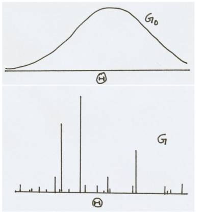
In the stick-breaking construction stick heights become shorter on average as we walk further down the number line. This means that earlier draws from the DP are more likely to be redrawn than later draws. When we use the DP to construct DPmem the memoized function will therefore tend to favor reuse of earlier computed values. Intuitively, we will use DPmem when we need to model reuse of samples in a scenario where we do not know in advance how many samples we need.

Infinite Mixture Models

We now return to the problem of categorization with an unknown number of categories. We can use the Dirichlet process to construct a distribution over an infinite set of (potential) bags:

(define colors '(blue green red))

(define samples
 (mh-query
   200 100

   (define phi (dirichlet '(1 1 1)))
   (define alpha 0.1)
   (define prototype (map (lambda (w) (* alpha w)) phi))

   (define bag->prototype (mem (lambda (bag) (dirichlet prototype))))

   ;;the prior distribution on bags is simply a DPmem of a gensym function:
   (define get-bag (DPmem 1.0 gensym))

   ;;each observation comes from one of the bags:
   (define obs->bag (mem (lambda (obs-name) (get-bag))))

   (define draw-marble
     (mem (lambda (obs-name)
            (multinomial colors (bag->prototype (obs->bag obs-name))))))

   ;;did obs1 and obs2 come from the same bag? obs1 and obs3?
   (list (equal? (obs->bag 'obs1) (obs->bag 'obs2))
         (equal? (obs->bag 'obs1) (obs->bag 'obs3)))

   (and
    (equal? 'red (draw-marble 'obs1))
    (equal? 'red (draw-marble 'obs2))
    (equal? 'blue (draw-marble 'obs3))
    (equal? 'blue (draw-marble 'obs4))
    (equal? 'red (draw-marble 'obs5))
    (equal? 'blue (draw-marble 'obs6))
    )))

(hist (map first samples) "obs1 and obs2 same category?")
(hist (map second samples) "obs1 and obs3 same category?")

A model like this is called an infinite mixture model; in this case an infinite Dirichlet-multinomial mixture model, since the observations (the colors) come from a multinomial distribution with Dirichlet prior. The essential addition in this model is that we have DPmem’d a gensym function to provide a collection of reusable category (bag) labels:

(define reusable-categories (DPmem 1.0 gensym))
(hist (repeat 20 reusable-categories))

To generate our observation in this infinite mixture model we first sample a category label from the memoized gensym. Since the Dirichlet process tends to reuse earlier choices (more than later ones), our data will tend to cluster together in earlier components. However, there is no a priori bound on the number of latent classes, rather there is just a bias towards fewer classes. The strength of this bias is controlled by the DP concentration parameter \(\alpha\). When \(\alpha\) is high, we will tolerate a larger number of classes, when it is low we will strongly favor fewer classes. In general, the number of classes grows proportional to \(\alpha \log(N)\) where \(N\) is the number of observations.

We can use this basic template to create infinite mixture models with any type of observation distribution. For instance here is an infinite Gaussian mixture model:

(define class-distribution (DPmem 1.0 gensym))

(define object->class
  (mem (lambda (object) (class-distribution))))

(define class->gaussian-parameters
  (mem (lambda (klass) (list  (gaussian 65 10) (gaussian 0 8)))))

(define (observe object)
  (apply gaussian (class->gaussian-parameters (object->class object))))

(map observe '(tom dick harry bill fred))

There are, of course, many possible observation models that can be used in the infinite mixture. One advantage of using abstract objects to represent our data is that we can associate different observation models with different aspects of the data. For instance, we could have a model which both models height and propensity to smoke for the same set of individuals, based on their sex.

Another View of the DP: The Chinese Restaurant Process

If you have looked at the literature on Bayesian models of cognition in the last few years, you will have seen many uses of a prior distribution known as the Chinese Restaurant Process. The Chinese Restaurant Process is an alternate, but equivalent, way to construct the Dirichlet process. The CRP is usually described as a sequential sampling scheme using the metaphor of a restaurant.

We imagine a restaurant with an infinite number of tables. The first customer enters the restaurant and sits at the first unoccupied table. The (\(N+1\))th customer enters the restaurant and sits at either an already occupied table or a new, unoccupied table, according to the following distribution. \[\tau^{(N+1)} | \tau^{(1)},..., \tau^{(N)},\alpha \sim \sum_{i=1}^{K} \frac{ y_i }{ N + \alpha } \delta_{\tau_{i}} + \frac{ \alpha }{ N + \alpha } \delta_{\tau_{K+1}}\] \(N\) is the total number of customers in the restaurant. \(K\) is the total number of occupied tables, indexed by \(1 \geq i \geq K\). \(\tau^{(j)}\) refers to the table chosen by the \(j\)th customer. \(\tau_i\) refers to \(i\)th occupied table in the restaurant. \(y_i\) is the number of customers seated at table \(\tau_i\); \(\delta_{\tau}\) is the \(\delta\)-distribution which puts all of its mass on table \(\tau\). \(\alpha \geq 0\) is the concentration parameter of the model.

In other words, customers sit at an already-occupied table with probability proportional to the number of individuals at that table, or at a new table with probability controlled by the parameter \(\alpha\).

Each table has a dish associated with it. Each dish \(v\) is a label on the table which is shared by all the customers at that table. When the first customer sits at a new table, \(\tau_i\), a dish is sampled from another distribution, \(\mu\), and placed on that table. This distribution, \(\mu\), is called the base distribution of the Chinese restaurant process, and is a parameter of the model. From then on, all customers who are seated at table \(\tau_i\) share this dish, \(v_{\tau_i}\).

The following animation demonstrates the Chinese restaurant process (click on it).

The CRP can be used to define a stochastic memoizer just as the Dirichlet process. We let the dish at each table be drawn from the underlying procedure. When we seat a customer we emit the dish labeling the table where the customer sat. To use a CRP as a memoization distribution we associate our underlying procedure with a set of restaurants—one for each combination of a procedure with its arguments. We let customers represent particular instances in which a procedure is evaluated, and we let the dishes labeling each table represent the values that result from those procedure applications. The base distribution which generates dishes corresponds to the underlying procedure which we have memoized.

When we seat a customer at an existing table, it corresponds to retrieving a value from the memory. Every customer seated at an existing table always returns the dish placed at that table when it was created. When we seat a customer at a new table it corresponds to computing a fresh value from our memoized random function and storing it as the dish at the new table. Another way of understanding the CRP is to think of it as defining a distribution over ways of partitioning \(N\) items (customers) into \(K\) partitions (tables), for all possible \(N\) and \(K\).

The probability of a particular partition of \(N\) customers over \(K\) tables is the product of the probabilities of the \(N\) choices made in seating those customers. It can easily be confirmed that the order in which elements are added to the partition components does not affect the probability of the final partition (i.e. the terms of the product can be rearranged in any order). Thus the distribution defined by a CRP is exchangeable.

The probability of a particular CRP partition can also be written down in closed form as follows. \[P(\vec{y})=\frac{\alpha^{K}\Gamma[\alpha]\prod_{j=0}^{K}\Gamma[y_{j}]}{\Gamma[\alpha+\sum_{j=0}^{K}y_{j}]}\] Where \(\vec{y}\) is the vector of counts of customers at each table and \(\Gamma(\cdot)\) is the gamma function, a continuous generalization of the factorial function. This shows that for a CRP the vector of counts is sufficient.

As a distribution, the CRP has a number of useful properties. In particular, it implements a simplicity bias. It assigns a higher probability to partitions which (1) have fewer customers, (2) have fewer tables, and (3) for a fixed number of customers \(N\), assign them to the smallest number of tables.

Thus the CRP favors simple restaurants and implements a rich-get-richer scheme. Tables with more customers have higher probability of being chosen by later customers. These properties mean that, all else being equal, when we use the CRP as a stochastic memoizer we favor reuse of previously computed values.

Example: Goldwater Model 1

(Adapted from Goldwater, S., Griffiths, T. L., and Johnson, M. (2009). A Bayesian framework for word segmentation: Exploring the effects of context. Cognition, 112:21–54)

(define phones '(a e i o u k t p g d b s th f))
(define phone-weights (dirichlet (make-list (length phones) 1)))

(define num-words 10)

(define (sample-phone)
  (multinomial phones phone-weights))

(define (sample-phone-sequence)
  (repeat (poisson 3.0) sample-phone))

(define sample-word
  (DPmem 1.0
         (lambda ()
           (sample-phone-sequence))))

(define (sample-utterance)
  (repeat num-words sample-word))

(sample-utterance)

Example: Infinite Hidden Markov Models

Just as when we considered a mixture model over an unknown number of latent categories, we may wish to have a hidden Markov model over an unknown number of latent symbols. We can do this by again using a reusable source of state symbols:

(define vocabulary '(chef omelet soup eat work bake))

(define (get-state) (DPmem 0.5 gensym))

(define state->transition-model
  (mem (lambda (state) (DPmem 1.0 (get-state)))))

(define (transition state)
  (sample (state->transition-model state)))

(define state->observation-model
  (mem (lambda (state) (dirichlet (make-list (length vocabulary) 1)))))

(define (observation state)
  (multinomial vocabulary (state->observation-model state)))

(define (sample-words last-state)
  (if (flip 0.2)
      '()
      (pair (observation last-state) (sample-words (transition last-state)))))

(sample-words 'start)

This model is known as the “infinite hidden Markov model”. Notice how the transition model uses a separate DPmemoized function for each latent state: with some probability it will reuse a transition from this state, otherwise it will transition to a new state drawn from the globally shared source or state symbols—a DPmemoized gensym.

Example: The Infinite Relational Model

(Adapted from: Kemp, C., Tenenbaum, J. B., Griffiths, T. L., Yamada, T. & Ueda, N. (2006). Learning systems of concepts with an infinite relational model. Proceedings of the 21st National Conference on Artificial Intelligence.)

Much semantic knowledge is inherently relational. For example, verb meanings can often be formalized as relations between their arguments. The verb “give” is a three-way relation between a giver, something given, and a receiver. These relations are also inherently typed. For example, the giver in the relation above is typically an agent. In a preceding section, we discussed the infinite mixture models, where observations were generated from a potentially unbounded set of latent classes. In this section we introduce an extension of this model to relational data: the infinite relational model (IRM).

Given some relational data, the IRM learns to cluster objects into classes such that whether or not the relation holds depends on the pair of object classes. For instance, we can imagine trying to infer social groups from the relation of who talks to who:

(define samples
  (mh-query
   300 100

   (define class-distribution (DPmem 1.0 gensym))

   (define object->class
     (mem (lambda (object) (class-distribution))))

   (define classes->parameters
     (mem (lambda (class1 class2) (beta 0.5 0.5))))

   (define (talks object1 object2)
     (flip (classes->parameters (object->class object1) (object->class object2))))

   (list (equal? (object->class 'tom) (object->class 'fred))
         (equal? (object->class 'tom) (object->class 'mary)))

   (and (talks 'tom 'fred)
        (talks 'tom 'jim)
        (talks 'jim 'fred)
        (not (talks 'mary 'fred))
        (not (talks 'mary 'jim))
        (not (talks 'sue 'fred))
        (not (talks 'sue 'tom))
        (not (talks 'ann 'jim))
        (not (talks 'ann 'tom))
        (talks 'mary 'sue)
        (talks 'mary 'ann)
        (talks 'ann 'sue)
        )))

(hist (map first samples) "tom and fred in same group?")
(hist (map second samples) "tom and mary in same group?")

We see that the model invents two classes (the “boys” and the “girls”) such that the boys talk to each other and the girls talk to each other, but girls don’t talk to boys. Note that there is much missing data (unobserved potential relations) in this example.

Example: CrossCat

(Adapted from: Shafto, P. Kemp, C., Mansignhka, V., Gordon, M., and Tenenbaum, J. B. (2006). Learning cross-cutting systems of categories. Proceedings of the Twenty-Eighth Annual Conference of the Cognitive Science Society.)

Often we have data where each object is associated with a number of features. In many cases, we can predict how these features generalize by assigning the objects to classes and predicting feature values on a class-by-class basis. In fact, we can encode this kind of structure using the IRM above if we interpret the relations as the presence of absence of a feature. However, in some cases this approach does not work because objects can be categorized into multiple categories, and different features are predicted by different category memberships.

For example, imagine we have some list of foods like: eggs, lobster, oatmeal, etc., and some list of features associated with these foods, such as: dairy, inexpensive, dinner, eaten with soup, etc. These features depend on different systems of categories that foods fall into, for example, one set of features may depend on the time of day that the foods are eaten, while another set may depend on whether the food is animal or vegetable based. CrossCat is a model designed to address these problems. The idea behind CrossCat is that features themselves cluster into kinds. Within each kind, particular objects will cluster into categories which predict the feature values for those objects in the kind. Thus CrossCat is a kind of hierarchical extension to the IRM which takes into account multiple domains of featural information.

(define kind-distribution (DPmem 1.0 (make-gensym "kind")))

(define feature->kind
  (mem (lambda (feature) (kind-distribution))))

(define kind->class-distribution
  (mem (lambda (kind) (DPmem 1.0 (make-gensym "class")))))

(define feature-kind/object->class
  (mem (lambda (kind object) (sample (kind->class-distribution kind)))))

(define class->parameters
  (mem (lambda (object-class) (beta 1 1))))

(define (observe object feature)
  (flip (class->parameters (feature-kind/object->class (feature->kind feature) object))))

(observe 'eggs 'breakfast)

Other Non-Parametric Distributions

The Dirichlet Process is the best known example of a non-parametric distribution. The term non-parametric refers to statistical models whose size or complexity can grow with the data, rather than being specified in advance (sometimes these are called infinite models, since they assumes an infinite, not just unbounded number of categories). There a number of other such distributions that are worth knowing.

Pitman-Yor Distributions

Many models in the literature use a small generalization of the CRP known as the Pitman-Yor process (PYP). The Pitman-Yor process is identical to the CRP except for having an extra parameter, \(a\), which introduces a dependency between the probability of sitting at a new table and the number of tables already occupied in the restaurant.

The process is defined as follows. The first customer enters the restaurant and sits at the first table. The (\(N+1\))th customer enters the restaurant and sits at either an already occupied table or a new one, according to the following distribution. \[ \tau^{(N+1)} | \tau^{(1)},...,\tau^{(N)}, a, b \sim \sum_{i=1}^{K} \frac{ y_i - a }{ N + b } \delta_{\tau_{i}} + \frac{ Ka + b }{ N + b } \delta_{\tau_{K+1}} \] Here all variables are the same as in the CRP, except for \(a\) and \(b\). \(b \geq 0\) corresponds to the CRP \(\alpha\) parameter. \(0 \leq a \leq 1\) is a new discount parameter which moves a fraction of a unit of probability mass from each occupied table to the new table. When it is \(1\), every customer will sit at their own table. When it is \(0\) the distribution becomes the single-parameter CRP. The \(a\) parameter can be thought of as controlling the productivity of a restaurant: how much sitting at a new table depends on how many tables already exist. On average, \(a\) will be the limiting proportion of tables in the restaurant which have only a single customer. The \(b\) parameter controls the rate of growth of new tables in relation to the total number of customers \(N\) as before.

Like the CRP, the sequential sampling scheme outlined above generates a distribution over partitions for unbounded numbers of objects. Given some vector of table counts \(\vec{y}\), A closed-form expression for this probability can be given as follows. First, define the following generalization of the factorial function, which multiples \(m\) integers in increments of size \(a\) starting at \(x\). \[ [x]_{m,s} = \begin{cases} 1 & \text{for } m=0 \\ x(x+s)...(x+(m-1)s)& \text{for } m > 0 \end{cases} \] Note that \([1]_{m,1} = m!\). The probability of the partition given by the count vector, \(\vec{y}\), is defined by: \[ P( \vec{y} \mid a, b) = \frac{[b+a]_{K-1,a}}{[b+1]_{N-1,1}} \prod_{i=1}^{K}[1-a]_{y_i-1,1} \] It is easy to confirm that in the special case of \(a = 0\) and \(b >0\), this reduces to the closed form for CRP by noting that \([1]_{m,1} = m! = \Gamma[m+1]\). In what follows, we will assume that we have a higher-order function PYmem which takes three arguments a, b, and proc and returns the PYP-memoized version of proc.

The Indian Buffet Process

The Indian Buffet Process is an infinite distribution on sets of draws from a base measure (rather than a single draw as in the CRP).

Hierarchical Combinations of Non-parametric Processes

In the Hierarchical Models chapter, we explored how additional levels of abstraction can lead to important effects in learning dynamics, such as transfer learning and the blessing of abstraction. In this section, we talk about two ways in which hierarchical non-parametric models can be built.

The Nested Chinese Restaurant Process

We have seen how the Dirichlet Process/CRP can be used to learn mixture models where the number of categories is infinite. However, the categories associated with each table or stick in the DP/CRP are unstructured, whereas real life categories have complex relationships with one another. For example, they are often organized into hierarchies: a German shepherd is a type of dog, which is a type of animal, which is type of living thing, and so on.

In Example: One-shot learning of visual categories, we saw how such hierarchies could lead to efficient one-shot learning, but we did not talk about how such a hierarchy itself could be learned. The Nested Chinese Restaurant Process (nCRP) is one way of doing this. (Blei, D. M., Griffiths, T. L., Jordan, M. I., and Tenenbaum, J. B, 2004. Hierarchical topic models and the nested chinese restaurant process. In Advances in Neural Information Processing Systems 16). The idea behind the nCRP is that tables in a CRP, which typically represent categories, can refer to other restaurants that represent lower-level categories.

(define top-gensym (make-gensym "t"))
(define top-level-category (DPmem 1.0 top-gensym))

(define subordinate-gensym (make-gensym "s"))
(define subordinate-category
  (DPmem 1.0
         (lambda (parent-category)
           (list (subordinate-gensym) parent-category))))

(define (sample-category) (subordinate-category (top-level-category)))

(table (pair (list "subordinate" "top")
             (repeat 10 sample-category)))

Each call to sample-category returns a list that consists of a subordinate-level category followed by the corresponding top-level category. These categories are represented by gensyms, and, because they are drawn from a DP-memoized version of gensym, there is no a priori limit on the number of possible categories at each level.

The nCRP gives us a way of constructing unbounded sets of hierarchically nested categories, but how can we use such structured categories to generate data? The code below shows one way:

(define top-gensym (make-gensym "t"))
(define possible-observations '(a b c d e f g))

(define top-level-category (DPmem 1.0 top-gensym))
(define top-level-category->parameters
  (mem (lambda (cat) (dirichlet (make-list (length possible-observations) 1.0)))))

(define subordinate-gensym (make-gensym "s"))
(define subordinate-category
  (DPmem 1.0
         (lambda (parent-category)
           (list (subordinate-gensym) parent-category))))

(define subordinate-category->parameters
  (mem (lambda (cat) (dirichlet (top-level-category->parameters (second cat)))))) 

(define (sample-category) (subordinate-category (top-level-category)))

(define (sample-observation) (multinomial possible-observations (subordinate-category->parameters (sample-category))))

(repeat 10 sample-observation)

This code shows a model where each category is associated with a multinomial distribution over the following possible observations: (a b c d e f g). This distribution is drawn from a Dirichlet prior for each subordinate-level category. However, the pseudocounts for the Dirichlet distribution for each subordinate-level category are drawn from another Dirichlet distribution which is associated with the top-level category—all of the subordinate level categories which share a top-level category also have similar distributions over observations.

In fact, the model presented in Example: One-shot learning of visual categories works in the same way, except that each category is associated with Gaussian distribution and the mean and variance parameters are shared between subordinate level categories.

The Hierarchical Dirichlet Process

In the last section, we saw an example where subordinate-level categories drew their hyperparameters from a shared Dirichlet distribution. It is also possible to build a similar model using a Dirichlet Process at each level. This model is known as the Hierarchical Dirichlet Process (HDP). (Teh, Y. W., Jordan, M. I., Beal, M. J., and Blei, D. M. (2006). Hierarchical dirichlet processes. Journal of the American Statistical Association, 101(476):1566–1581.)

(define base-measure (lambda () (poisson 20)))
(define top-level  (DPmem 10.0 base-measure))
(define sample-observation
  (DPmem 1.0
         (lambda (component)
           (top-level))))

(hist (repeat 1000 base-measure) "Draws from Base Measure (poisson 20)")
(hist (repeat 1000 top-level) "Draws from Top Level DP")
(hist (repeat 1000 (lambda () (sample-observation 'component1))) "Draws from Component DP 1")
(hist (repeat 1000 (lambda () (sample-observation 'component2))) "Draws from Component DP 2")
(hist (repeat 1000 (lambda () (sample-observation 'component3))) "Draws from Component DP 3")

In an HDP, there are several component Dirichlet Processes (labeled here as component1, component2, etc.). These component DPs all share another DP (called top-level) as their base measure.

In the example above, we have used a poisson distribution as the base measure. The top-level DP concentrates this distribution into a number of points. Each of the component DPs then further concentrate this distribution—sharing the points chosen by the top-level DP, but further concentrating it, each in their own way.

A natural move is to combine the nCRP and HDP: the nCRP can be used to sample an unbounded set of hierarchically structured categories, and the HDP can be used to make these categories share observations in interesting ways.

(define top-gensym (make-gensym "t"))
(define top-level-category (DPmem 1.0 top-gensym))

(define root-category (DPmem 10.0 (lambda () (poisson 20))))

(define sample-from-top-level-category (DPmem 1.0 (lambda (cat) (root-category))))

(define subordinate-gensym (make-gensym "s"))
(define subordinate-category
  (DPmem 1.0
         (lambda (parent-category)
           (list (subordinate-gensym) parent-category))))

(define (sample-category) (subordinate-category (top-level-category)))

(define sample-observation
  (DPmem 1.0
         (lambda (cat)
           (sample-from-top-level-category (rest cat)))))

(repeat
 10
 (lambda ()
   (let* ([category (sample-category)]
          [subordinate (first category)]
          [top (second category)]
          [h1 (hist (repeat 1000 (lambda () (sample-observation category)))
                    (string-append  "Top Level: " top ", Subordinate Level: " subordinate))]
          [h2 (hist (repeat 1000 (lambda () (sample-from-top-level-category top)))
                    (string-append  "Top Level: " top))]
          [h3 (hist (repeat 1000 (lambda () (sample-observation category)))
                    "Root Category")])
     'dummy)))

Note that the nCRP and the HDP represent very different ways to construct distributions with hierarchically arranged non-parametric distributions. The nCRP builds a hiearchy of category types, while the HDP shares observations between multiple DPs.

Example: Prototypes and Exemplars

An important debate in psychology and philosophy has concerned the nature of concepts. The classical theory of concepts holds that they can defined in terms of necessary and sufficient conditions. For example, the concept dog might consist of a list of features— such as furry, barks, etc. If an object in the world matches the right features, then it is a dog.

However, it appears that, at least for some concepts, the classical theory faces some difficulties. For example, some concepts appear to be family resemblance categories (FRC). Members of a FRC share many features in commone, but the overlap is not total, and there is the possibility that two members of the category can share no feature in common, instead, each sharing features with other members of the category.

The philosopher Wittgenstein—who introduced the concept of Family Resemblance Categories—famously discussed the example of games. There are many different kinds of games: ball games, drinking games, children’s playground games, card games, video games, role-playing games, etc. It is not clear that there is a single list of features which they all share and which can uniquely identify them all as game (See: Murphy, G. L. 2004. The Big Book of Concepts. The MIT Press. For an in-depth discussion of many issues surrounding concepts.).

Two theories have emerged to explain FRCs (and other related phenomena): prototype theories and exemplar theories. In prototype theories, concepts are considered to be based on a single stored prototype. People judge whether something is an example of a concept by comparing to this stored representation. For example, the prototype for dog might include features such as furry, barks, etc. An object is a member of a category (concept) to the degree that it matches the single stored prototype.

In exemplar theories, by contrast, it is assumed that people store all examples of a particular concept, rather than a single summary representation in prototype forms. A new object is classified by comparison with all of these forms.

Both prototype and exemplar theories are based on similarity, and the probability that an observation is assigned to category \(c_{N}\) can be given by \[p(c_{N} \mid x_N, \vec{x}_{N-1}, \vec{c}_{N-1}) = \frac{\eta_{N,j}\beta_{N,j}}{\sum_{c} \eta_{N,c}\beta_{N,c}}\] where \(\eta_{N,i}\) is the similarity between observation \(N\) and category \(i\), and \(\beta_{N,i}\) is the response bias for the category (i.e., its prior weight).

Exemplar models treat the similarity between observation \(N\) and a category as a sum over all members of the category: \[\eta_{N,i} = \sum_{i \mid c_{i} = j } \eta_{N,i}\] Prototype models treat the similarity as the similarity between observation \(N\) and the single stored prototype: \[\eta_{N,i} = \eta_{N,p_i}\] Notice that these two models can be seen as opposite ends of a spectrum; one estimates the category based on every member, while the other estimates based on a single member. There are clearly many intermediate points where each category can be viewed as a mixture over \(K\) clusters.

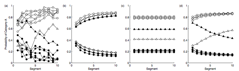
Griffiths et al. (2007) show how a large number of different models of categorization can be unified by viewing them all as special cases of a HDP which learns how many clusters each category should be represented by. (Griffiths, T. L., Canini, K. R., Sanborn, A. N., and Navarro, D. J. (2007). Unifying rational models of categorization via the hierarchical dirichlet process. In Proceedings of the Twenty-Ninth Annual Conference of the Cognitive Science Society.)

In particular, Griffiths et al. (2007) examine the data from Smith and Minda (1998), which shows how learners undergo a transition from ptototype to exemplar representations during the course of learning. (Smith, J. D. and Minda, J. P. (1998). Prototypes in the mist: The early epochs of category learning. Journal of Experimental Psychology: Learning, Memory, and Cognition)

The results are shown below.