10. Occam’s Razor
Entities should not be multiplied without necessity. –William of Ockham
In learning, perceiving or thinking about the world, we are fitting models to the data of experience. Typically our hypothesis space will span models varying greatly in complexity: some models will have many more free parameters or degrees of freedom than others. Under traditional approaches to model fitting where we adjust each model’s parameters until it fits best, then choose the best-fitting model — a model with strictly more free parameters will tend to be preferred regardless of whether it actually comes closer to describing the true processes that generated the data. But this is not the way the mind works. We assess models with a natural eye for complexity, balancing fit to the data with model complexity in subtle ways that will not inevitably prefer the most complex model. Instead we often seem to judge models using Occam’s razor: we choose the least complex hypothesis that fits the data well. In doing so we avoid “over-fitting” our data in order to support successful generalizations and predictions.
Fitting curves (or smooth functions) to sparsely sampled, noisy data provides a familiar example of the problem.
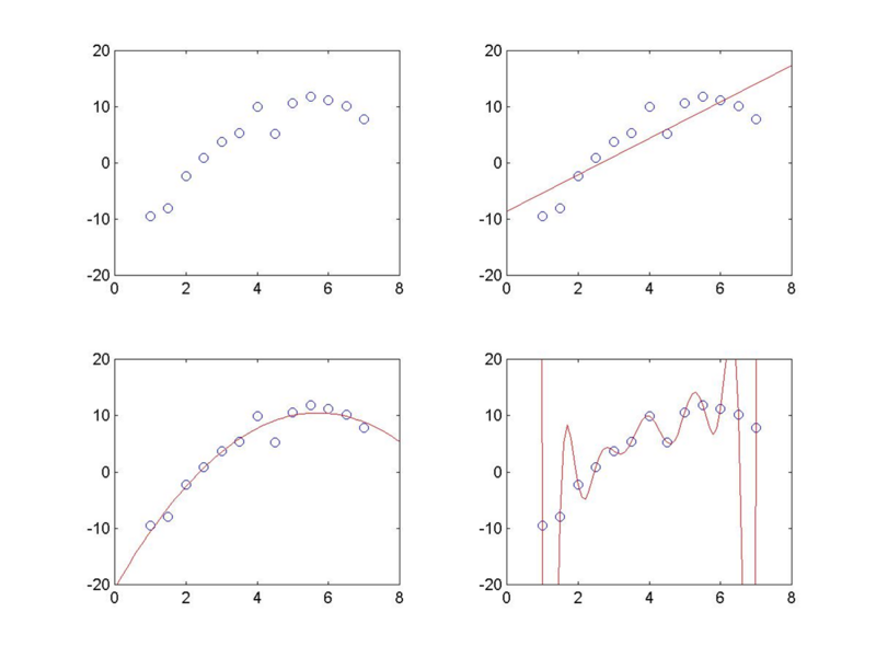
The figure above shows three polynomial fits: a 1st-order (linear), a 2nd-order (quadratic), and a 12th-order polynomial. How do our minds decide which of these functions provides the best account of the data? The 1st-order model captures the rough trend of the data but seems too coarse; it attributes some of the variation that we see as “signal” to “noise”. The 2nd-order model seems best; it seems to be just complex enough to fit the main shape of the data without over-fitting the noise. The 12th-order model seems ridiculously over-fit; with 13 data points, the parameters can be adjusted so as to make the curve pass exactly through every data point, thus taking as “signal” all of what we see as “noise”. Again we can think of this as a causal inference problem: each function represents a hypothesis about the causal process that gave rise to the observed data, including the shape of the function from inputs to outputs, as well as the level of noise added to the output.
Occam’s Razor
An elegant and powerful form of Occam’s razor arises in the context of Bayesian inference, known as the Bayesian Occam’s razor. Bayesian Occam’s razor refers to the fact that “more complex” hypotheses about the data are penalized automatically in conditional inference. In many formulations of Occam’s razor, complexity is measured syntactically: for instance, it may be the description length of the hypothesis in some representation language, or a count of the number of free parameters needed to pick out the hypothesis from some larger model class. Syntactic forms of Occam’s razor have difficulty justifying the complexity measure on principled, non-arbitrary grounds. They also leave unspecified exactly how the weight of a complexity penalty should trade off with an alternative measure of fit to the data. Fit is intrinsically a semantic notion, a matter of correspondence between the model’s predictions and our observations of the world. When complexity is measured syntactically and fit is measured semantically, they are intrinsically incommensurable and the trade-off between them will always be to some extent arbitrary.
In the Bayesian Occam’s razor, both complexity and fit are measured semantically. The semantic notion of complexity is a measure of flexibility: a hypothesis that is flexible enough to generate many different sets of observations is more complex, and will tend to receive lower posterior probability than a less flexible, simpler hypothesis that explains the same data. Because more complex hypotheses can generate a greater variety of data sets, they must necessarily assign a lower probability to each one. When we condition on some data, all else being equal, the posterior distribution over the hypotheses will favor the simpler ones because they have the tightest fit to the observations.
From the standpoint of a sampling-based probabilistic programming language such as Church, the Bayesian Occam’s razor is essentially inescapable. We do not judge models based on their best fitting behavior but rather on their average behavior. No fitting per se occurs during conditional inference. Instead, we draw conditional samples from each model representing the model’s likely ways of generating the data. A model that tends to fit the data well on average – to produce relatively many generative histories with that are consistent with the data – will do better than a model that can fit better only for atypical parameter settings but worse on average.
The Law of Conservation of Belief
It is convenient to emphasize an aspect of probabilistic modeling that seems deceptively trivial, but comes up repeatedly when thinking about inference. In Bayesian statistics we think of probabilities as being degrees of belief. Our generative model reflects world knowledge and the probabilities that we assign to the possible sampled values reflect how strongly we believe in each possibility. The laws of probability theory ensure that our beliefs remain consistent as we reason.
A consequence of belief maintenance is known as the Law of Conservation of Belief (LCB). Here are two equivalent formulations of this principle:
- Sampling from a distribution selects exactly one possibility (in doing so it implicitly rejects all other possible values).
- The total probability mass of a distribution must sum to \(1\). That is, we only have a single unit of belief to spread around.
The latter formulation leads to a common metaphor in discussing generative models: We can usefully think of belief as a “currency” that is “spent” by the probabilistic choices required to construct a sample. Since each choice requires “spending” some currency, an outcome that requires more choices to construct it will generally be more costly, i.e. less probable.
It is this conservation of belief that gives rise to the Bayesian Occam’s razor. A hypothesis that spends its probability on many alternatives that don’t explain the current data will have less probability for the alternatives that do, and will hence do less well overall than a hypothesis which only entertains options that fit the current data. We next examine a special case where this tradeoff plays out clearly, the size principle, then come back to the more general cases.
The Size Principle
A simple case of Bayes Occam’s razor comes from the size principle (Tenenbaum & Griffiths, 2001): Of hypotheses which generate data uniformly, the one consistent with the data and with smallest extension is the most probable.
The following Church program demonstrates the size principle with a very simple model. Here we have two hypothesized sets: Big has 6 elements and Small has 3 elements. The generative model chooses one of the hypotheses at random and samples some number of symbols from it uniformly. We then wish to infer the hypothesis given observed elements.
(define samples
   (mh-query
    100 100

    (define (hypothesis->set  hyp)
      (if (equal? hyp  'Big) '(a b c d e f) '(a b c)))

    (define hypothesis (if (flip) 'Big 'Small))
    (define (observe N)
      (repeat N (lambda () (uniform-draw (hypothesis->set hypothesis)))))

    hypothesis

    (equal? (observe 1) '(a))
    )
   )
 (hist samples "Size Principle")
With a single observed a, we already favor hypothesis Small. What happens when we increase the amount of observed data? Consider the learning trajectory:
(define (samples data)
   (mh-query
    100 10

    (define (hypothesis->set  hyp)
      (if (equal? hyp  'Big) '(a b c d e f) '(a b c)))

    (define hypothesis (if (flip) 'Big 'Small))
    (define (observe N)
      (repeat N (lambda () (uniform-draw (hypothesis->set hypothesis)))))

    hypothesis

    (equal? (observe (length data)) data)
    )
   )

(define (big-freq data) (mean (map (lambda (hyp) (if (equal? hyp 'Big) 1.0 0.0)) (samples data))))

(lineplot
 (list
  (pair 1 (big-freq '(a)))
  (pair 3 (big-freq '(a b a)))
  (pair 5 (big-freq '(a b a b b)))
  (pair 7 (big-freq '(a b a b b a b))))
 "P(Big | observations)"
 )
As the number of data points increases, the hypothesis Small rapidly comes to dominate the posterior distribution. Why is this happening? We sample observations uniformly from hypotheses, the law of conservation of belief and the symmetry between observations imply that the probability of a draw from Big is \(\frac{1}{6}\), while the probability of a draw from Small is \(\frac{1}{3}\). Thus, by the product rule of probabilities, the probability of drawing a set of N observations from Big is \((\frac{1}{6})^N\), while the probability of drawing a set of observations from Small is \((\frac{1}{3})^N\). The later probability decreases much more slowly than the former as the number of observations increases. Using Bayes’ rule, the posterior distribution over hypotheses is given by:
\[P(\text{hypothesis} \mid \text{observations}) \propto P(\text{observations} \mid \text{hypothesis})P(\text{hypothesis})\]
Because our hypotheses are equally probable a priori, this simplifies to:
\[P(\text{hypothesis} \mid \text{observations}) \propto P(\text{observations} \mid \text{hypothesis})\]
So we see that the the posterior distribution over hypotheses in this case is just the normalized likelihood \(P(\text{observations} \mid \text{hypothesis})\). The likelihood ratio \(P(\text{observations} \mid \text{Big})/P(\text{observations} \mid \text{Small}) = (\frac{1}{2})^N\) determines how quickly the simpler hypothesis Small comes to dominate the posterior.
The size principle is related to an influential proposal in linguistics known as the subset principle. Intuitively, the subset principle suggests that when two grammars both account for the same data, the grammar that generates a smaller language should be preferred.1
Example: The Rectangle Game
Note: This example is still being ported from the old tutorial; it does not currently run
To illustrate the power of the size principle in inferring the most parsimonious explanation of data, consider learning a rectangle “concept” Tenenbaum, 2000. The data are a set of point in the plane, that we assume to be randomly sampled from within some unknown rectangle. Given the examples, what is the rectangle they came from? We can model this learning as conditional of the rectangle given the points. We plot the sampled rectangles as well as the posterior mean:
;;observed points:
(define obs-data '((0.4 0.7) (0.5 0.4) (0.46 0.63) (0.43 0.51)))

;;parameters and helper functions:
(define noise 0.001)
(define num-examples (length obs-data))

;;infer the rectangle given the observed points:
;;observed points:
(define obs-data '((0.4 0.7) (0.5 0.4) (0.46 0.63) (0.43 0.51)))

;;parameters and helper functions:
(define noise 0.001)
(define num-examples (length obs-data))

;;infer the rectangle given the observed points:
(define samples
  (drop
   (mh-query
    300 100

    ;;sample the rectangle
    (define x1 (uniform 0 1))
    (define x2 (uniform 0 1))
    (define y1 (uniform 0 1))
    (define y2 (uniform 0 1))

    ;;the concept is uniform over this rectangle
    (define concept
      (lambda () (list (uniform x1 x2) ;;x-val uniform in rect
                       (uniform y1 y2) ;;y-val uniform in rect
                       )))

    (list x1 x2 y1 y2)

    (map (lambda (example) (condition (equal? (uniform x1 x2) (first example)))) obs-data)
    (map (lambda (example) (condition (equal? (uniform y1 y2) (second example)))) obs-data))

  100))

;;set up fancy graphing:
(define (adjust points)
  (map (lambda (p) (+ (* p 350) 25))
       points))
(define paper (make-raphael "my-paper" 400 400))
(define (draw-rect rect color alpha linewidth)
  (let* ((rect (adjust rect))
         (x-lower (min (first rect) (second rect)))
         (y-lower (min (third rect) (fourth rect)))
         (width (abs (- (second rect) (first rect))))
         (height (abs (- (fourth rect) (third rect)))))
    (raphael-js paper
      "rect = r.rect(" x-lower ", " y-lower ", " width ", " height
      "); rect.attr('stroke', " color
      "); rect.attr('stroke-width', " linewidth
      "); rect.attr('stroke-opacity', " alpha ")")))

;;graph the observed points:
(raphael-points paper
                (adjust (map first obs-data))
                (adjust (map second obs-data)))

;;graph the sampled rectangles:
(map (lambda (rect) (draw-rect rect "'aaa'" 0.1 0.5)) samples)

;;graph the mean rectangle:
(define mean-bounds (map mean (list (map first samples) (map second samples) (map third samples) (map fourth samples))))
(draw-rect mean-bounds "'#1f3'" 1 3)

(draw-rect (list 0 1 0 1) "'#000'" 1 2)

'done
Explore how the concept learned varies as a function of the number and distribution of example points. Try varying the observed data and seeing how the inferred rectangle changes:
(define obs-data '((0.2 0.6) (0.2 0.8) (0.4 0.8) (0.4 0.6) (0.3 0.7)))
(define obs-data '((0.4 0.7) (0.5 0.4) (0.45 0.5) (0.43 0.7) (0.47 0.6)))
(define obs-data '((0.4 0.7) (0.5 0.4)))
(define obs-data '((0.4 0.7) (0.5 0.4) (0.46 0.63) (0.43 0.51) (0.42 0.45) (0.48 0.66)))
Compare this to the results of a slightly different causal process for the same observations, known as weak sampling:
;;observed points (now points and in/out labels):
(define obs-data '((0.4 0.7 #t) (0.5 0.4 #t) (0.46 0.63 #t) (0.43 0.51 #t)))

;;parameters and helper functions:
(define num-examples (length obs-data))

;;infer the rectangle given the observed points:
(define samples
  (drop
   (mh-query
    300 100

    ;;sample the rectangle
    (define x1 (uniform 0 1))
    (define x2 (uniform 0 1))
    (define y1 (uniform 0 1))
    (define y2 (uniform 0 1))

    ;;the concept is now a rule for classifying points as in or out of this rectangle
    ;;we return both the point and the label
    (define (concept p)
      (list (first p)
            (second p)
            (and (< (first p) x2)
                 (> (first p) x1)
                 (< (second p) y2)
                 (> (second p) y1))))

    (list x1 x2 y1 y2)

    ;;condition on all the observed points being in the rectangle
    (all
      (map (lambda (datum) (equal? (third (concept (list (first datum) (second datum)))) (third datum)))
        obs-data)))

  100))

;;set up fancy graphing:
(define (adjust points)
  (map (lambda (p) (+ (* p 350) 25))
       points))
(define paper (make-raphael "my-paper" 400 400))
(define (draw-rect rect color alpha linewidth)
  (let* ((rect (adjust rect))
         (x-lower (min (first rect) (second rect)))
         (y-lower (min (third rect) (fourth rect)))
         (width (abs (- (second rect) (first rect))))
         (height (abs (- (fourth rect) (third rect)))))
    (raphael-js paper
      "rect = r.rect(" x-lower ", " y-lower ", " width ", " height
      "); rect.attr('stroke', " color
      "); rect.attr('stroke-width', " linewidth
      "); rect.attr('stroke-opacity', " alpha ")")))

;;graph the observed points:
(raphael-points paper
                (adjust (map first obs-data))
                (adjust (map second obs-data)))

;;graph the sampled rectangles:
(map (lambda (rect) (draw-rect rect "'aaa'" 0.1 0.5)) samples)

;;graph the mean rectangle:
(define mean-bounds (map mean (list (map first samples) (map second samples) (map third samples) (map fourth samples))))
(draw-rect mean-bounds "'#1f3'" 1 3)

(draw-rect (list 0 1 0 1) "'#000'" 1 2)

'done
The Size Principle and Implicit Negative Evidence
One way to understand the Size Principle is that probabilistic inference takes into account implicit negative evidence. More flexible hypotheses could have generated more observations. Thus if those hypotheses were the true hypotheses we would expect to see a greater variety of observations. If the data does not contain them, this is a form of negative evidence against those hypotheses. Importantly, the Size Principle tells us that the prior distribution on hypotheses does not have to penalize complexity. The complexity of the hypothesis itself will lead to its being disfavored in the posterior distribution.
Generalizing the Size Principle: Bayes Occam’s Razor
In our example above we have illustrated Bayes Occam’s razor with examples based strictly on the “size” of the hypotheses involved, however, the principle is more general. Bayes’ Occam razor says that all else being equal the hypothesis that assigns the highest likelihood to the data will dominate the posterior. Because of the law of conservation of belief, assigning higher likelihood to the observed data requires assigning lower likelihood to other possible data. Consider the following example
(define observed-letters '(a b a b c d b b))

(define samples
   (mh-query
    100 100

    (define (hypothesis->parameters hyp)
      (if (equal? hyp 'A)
          (list '(a b c d) '(0.375 0.375 0.125 0.125))
          (list '(a b c d) '(0.25 0.25 0.25 0.25))))

    (define hypothesis (if (flip) 'A 'B))

    (define (observe observed-letters)
      (map (lambda (letter) (condition (equal? (multinomial
              (first (hypothesis->parameters hypothesis))
              (second (hypothesis->parameters hypothesis)))
            letter)))
        observed-letters))

    hypothesis

    (observe observed-letters)

    )
   )

(hist samples "Bayes-Occam-Razor")
In this example, unlike the size principle cases above, both hypotheses lead to the same possible observed values. However, hypothesis A is skewed toward examples a and b—while it can produce c or d, it is less likely to do so. In this sense hypothesis A is less flexible than hypothesis B. The data set we conditioned on also has exemplars of all the elements in the support of the two hypotheses. However, because there are more exemplars of elements favored by hypothesis A, this hypothesis is favored in the posterior. The Bayesian Occam’s razor emerges naturally here, and is often described as favoring the less flexible hypothesis.
Similar effects emerge if hypothesis B is not uniform, but favors different examples that hypothesis A:
(define observed-letters '(a b a c d))

(define samples
   (mh-query
    100 100

    (define (hypothesis->parameters hyp)
      (if (equal? hyp 'A)
          (list '(a b c d) '(0.375 0.375 0.125 0.125))
          (list '(a b c d) '(0.25 0.25 0.25 0.25))))

    (define hypothesis (if (flip) 'A 'B))

    (define (observe observed-letters)
      (map (lambda (letter) (condition (equal? (multinomial
              (first (hypothesis->parameters hypothesis))
              (second (hypothesis->parameters hypothesis)))
            letter)))
        observed-letters))

    hypothesis

    (observe observed-letters)

    )
   )

(hist samples "Bayes-Occam-Razor")
Try changing the observed letters to d c d a b. How does the inference change? Note that it takes less evidence here to favor hypothesis A that when B is uniform, but still more that in a size principle case (where A wouldn’t be able to generate c or d at all)—but the size principle case would be unable to handle the “exceptional” observations of c and d. This examples suggest another way to understand Bayes Occam’s razor: the posterior distribution will favor hypotheses for which the data set is simpler in the sense that it is more “easily generated.” Here more “easily” generated, means generated with higher probability. We will see a more striking example of this for compositional models at the end of this section of the tutorial.
Model selection with the Bayesian Occam’s Razor
The law of conservation of belief turns most clearly into Occam’s Razor when we consider models with more internal structure: some continuous or discrete parameters that at different settings determine how likely the model is to produce data that look more or less like our observations. To select among models we simply need to describe each model as a probabilistic program, and also to write a higher-level program that generates these hypotheses. Church query will then automatically draw samples at both of these levels of abstraction, asking which models are most likely to have given rise to the observed data, as well as for each of those models, which internal parameter settings are most likely. Note that we are dealing with statistical models, which are stochastic, rather than deterministic.
Example: Fair or unfair coin?
In the previous section we considered learning about the weight of a coin, and noted that a simple prior on weights seemed unable to capture our more discrete intuition that we first decide if the coin if fair or not, and only then worry about its weight. This example shows how our inferences about coin flipping can be explained in terms of model selection guided by the Bayesian Occam’s razor. Imagine a coin that you take out of a freshly unwrapped roll of quarters straight from the bank. Almost surely this coin is fair… But how does that sense change when you see more or less anomalous sequences of flips? We can simultaneously ask if the coin is fair, and what is its weight.
;; fair coin, probability of H = 0.5
(define observed-data '(h h t h t h h h t h))

;; ?? suspicious coincidence, probability of H = 0.5 ..?
;; (define observed-data '(h h h h h h h h h h))

;; probably unfair coin, probability of H near 1
;; (define observed-data '(h h h h h h h h h h h h h h h))

;; definitely unfair coin, probability of H near 1
;; (define observed-data '(h h h h h h h h h h h h h h h h h h h h))

;; unfair coin, probability of H = 0.85
;; (define observed-data '(h h h h h h t h t h h h h h t h h t h h h h h t h t h h h h h t h h h h h h h h h t h h h h t h h h h h h h))

(define num-flips (length observed-data))
(define num-samples 1000)
(define fair-prior 0.999)
(define pseudo-counts '(1 1))

(define prior-samples
   (repeat num-samples
     (lambda () (if (flip fair-prior)
                     0.5
                    (beta (first pseudo-counts) (second pseudo-counts))))))

(define samples
   (mh-query
     num-samples 10

     (define fair-coin? (flip fair-prior))
     (define coin-weight (if fair-coin?
                             0.5
                             (beta (first pseudo-counts) (second pseudo-counts))))

     (define make-coin (lambda (weight) (lambda () (if (flip weight) 'h 't))))

     (list (if fair-coin? 'fair 'unfair) coin-weight)

     (map (lambda (datum) (condition (equal? (flip coin-weight) (equal? datum 'h)))) observed-data)
   )
)

(hist (map first samples) "Fair coin?")
(density (append '(0) '(1) prior-samples) "Coin weight, prior to observing data")
(density (append '(0) '(1) (map second samples)) "Coin weight, conditioned on observed data")
Try some of the other cases that we’ve commented out above and see if the inferences accord with your intuitions.
Now let’s look at the learning trajectories for this model:
(define make-coin (lambda (weight) (lambda () (if (flip weight) 'h 't))))

(define fair-prior 0.999)
(define pseudo-counts '(1 1))

(define (samples data)
  (mh-query 400 10

     (define fair-coin? (flip fair-prior))
     (define coin-weight (if fair-coin?
                             0.5
                            (beta (first pseudo-counts) (second pseudo-counts))))

     (define coin (make-coin coin-weight))

     coin-weight

     (map (lambda (datum) (condition (equal? (flip coin-weight) (equal? datum 'h)))) data)
   )
)

(define true-coin (make-coin 0.9))
(define full-data-set (repeat 100 true-coin))
(define observed-data-sizes '(1 3 6 10 20 30 50 70 100))
(define (estimate N) (mean (samples (take full-data-set N))))

(lineplot (map (lambda (N)
       (list N (estimate N)))
     observed-data-sizes))
In general (though not on every run) the learning trajectory stays near 0.5 initially—favoring the simpler hypothesis that the coin is fair—then switches fairly abruptly to near 0.9—as it infers that it is an unfair coin and likely has high weight. Here the Bayesian Occam’s Razor penalizes the hypothesis with the flexibility to learn any coin weight: we automatically get a notion of comparing the complexity of very differently-structured models.
The Effect of Unused Parameters
When statisticians suggest methods for model selection, they often include a penalty for the number of parameters (e.g., AIC). This seems like a worrying policy from the point of view of a probabilistic program: we could always introduce parameters that are not used, and therefore have no effect on the program. For instance we could change the above coin flipping example so that it draws the potential unfair coin weight even in the model which gives a fair coin:
(define make-coin (lambda (weight) (lambda () (if (flip weight) 'h 't))))

(define observed-data '(h))
(define fair-prior 0.5)

(define samples
   (mh-query
     1000 10

     (define unfair-coin-weight (beta 1 10))

     (define fair-coin? (flip fair-prior))
     (define coin-weight (if fair-coin?
                             0.5
                             unfair-coin-weight
                             ))

     (define coin (make-coin coin-weight))

     (list (if fair-coin? 'fair 'unfair) coin-weight)

     (map (lambda (datum) (condition (equal? (flip coin-weight) (equal? datum 'h)))) observed-data)
   )
)

(hist (map first samples) "Fair coin?")
The two models now have the same number of free parameters (the unfair coin weight), but we will still favor the simpler hypothesis, as we did above. Why? The Bayesian Occam’s razor penalizes models not for having more parameters (or longer code) but for too much flexibility — being able to fit too many other potential observations. Unused parameters (or parameters with very little effect) don’t increase this flexibility, and hence aren’t penalized. The Bayesian Occam’s razor only penalizes complexity that matters for prediction, and only to the extent that it matters.
Example: Curve Fitting
Note: This example is still being ported from the old tutorial; it does not currently run
This example shows how the Bayesian Occam’s Razor can be used to select the right order of a polynomial fit. This Church program samples polynomials up to order 3 that are (noisily) consistent with the observed data, then graphs the mean polynomial of each order.
;;first a helper function that makes a polynomial function, given the coefficients:
(define (make-poly c)
  (lambda (x) (apply + (map (lambda (a b) (* a (expt x b))) c (iota (length c))))))

;;now set up the observed data:
(define x-vals (range -5 5))
(define obs-y-vals '(-0.199 -0.208 -0.673 -0.431 -0.360 -0.478 -0.984 0.516 1.138 2.439 3.501))

;;y-vals generated from:
;(define true-y-vals (map (make-poly '(-.5 0.3 .1)) x-vals))
;(define obs-y-vals (map (lambda (x) (gaussian x 0.4)) true-y-vals))

(define (noisy-equals? x y)
  (log-flip (* -1000 (expt (- x y) 2))))

;;the actual curve inference:
(define samples
  (mh-query
   400 20

   (define poly-order (sample-integer 4))
   (define coefficients (repeat (+ poly-order 1) (lambda () (gaussian 0.0 2.0))))

   (define y-vals (map (make-poly coefficients) x-vals))

   (list poly-order coefficients)

   (all (map noisy-equals? y-vals obs-y-vals))
   )
  )

;;now let's look at the results:
(hist (map first samples) "Polynomial degree")

;;find the average coefficients for sampled polynomials of each order:
(define (mean-coeffs order)
  (let ((coeffs (map second (filter (lambda (s) (= order (first s))) samples))))
    (if (null? coeffs)
        '()
        (map (lambda (c) (mean c)) (apply zip coeffs)))))


;;set up graphing:
(define plot-x-vals (map (lambda (x) (/ x 10)) (range -50 50)))
(define plot-0-y-vals (map (make-poly (mean-coeffs 0)) plot-x-vals))
(define plot-1-y-vals (map (make-poly (mean-coeffs 1)) plot-x-vals))
(define plot-2-y-vals (map (make-poly (mean-coeffs 2)) plot-x-vals))
(define plot-3-y-vals (map (make-poly (mean-coeffs 3)) plot-x-vals))

(define (adjust points)
  (map (lambda (p) (+ (* (+ p 5) 25) 25))
       points))

;; 0th order polynomial
(define paper-0 (make-raphael "polynomial-0" 250 250))
(raphael-points paper-0 (adjust x-vals) (adjust obs-y-vals))
(raphael-lines paper-0 (adjust plot-x-vals) (adjust plot-0-y-vals))

;; 1st order polynomial
(define paper-1 (make-raphael "polynomial-1" 250 250))
(raphael-points paper-1 (adjust x-vals) (adjust obs-y-vals))
(raphael-lines paper-1 (adjust plot-x-vals) (adjust plot-1-y-vals))

;; 2nd order polynomial
(define paper-2 (make-raphael "polynomial-2" 250 250))
(raphael-points paper-2 (adjust x-vals) (adjust obs-y-vals))
(raphael-lines paper-2 (adjust plot-x-vals) (adjust plot-2-y-vals))

;; 3rd order polynomial
(define paper-3 (make-raphael "polynomial-3" 250 250))
(raphael-points paper-3 (adjust x-vals) (adjust obs-y-vals))
(raphael-lines paper-3 (adjust plot-x-vals) (adjust plot-3-y-vals))

'done
Try the above code using a different data set generated from the same function:
(define obs-y-vals '(0.66 -0.32 -0.41 -0.59 -0.87 -0.75 -0.23 0.47 1.31 1.97 3.25))Try a simpler data set that should also suggest a 2nd order polynomial:
(define x-vals (range -3 3))
(define obs-y-vals '(2 0.1 -1 -1.5 -0.8 0 1.9))
These data should suggest a 1st order polynomial:
(define x-vals (range -3 3))
(define obs-y-vals '(2 1.6 0.9 0.3 -0.1 -0.45 -1.2))
Example: Scene Inference
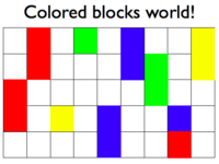
Imagine you are in a world of colored blocks that typically looks something like this:
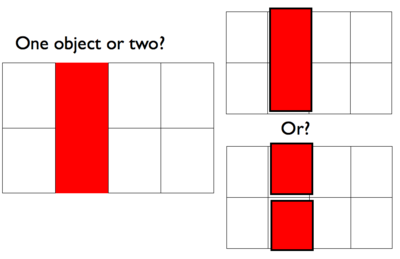
And one day you see this 1x2 red patch… is it one 1x2 block or two 1x1 blocks?
We can model this inference by building a generative model of scenes. To do so we use simple models of geometry and of rendering geometric objects to an image (in this case by layering them):
;;take an object and "render" it into an image (represented as a list of lists):
(define (object-appearance object)
  (map (lambda (pixel-y)
         (map (lambda (pixel-x) (if (or (< pixel-x (first object))
                                        (<= (+ (first object) 1) pixel-x)
                                        (< pixel-y (second object))
                                        (<= (+ (second object) (third object)) pixel-y))
                                    0
                                   (fourth object)))
              '(0 1 2 3)))
         '(0 1)))

;;layer the image of an object onto a "background" image. Note that the object occludes the background.
(define (layer object image) (map (lambda (obj-row im-row)
                                    (map (lambda (o i) (if (= 0 o) i o))
                                         obj-row
                                         im-row))
                                  object image))

;;prior distribution over objects' properties:
(define (sample-properties)
  (list (sample-integer 4) ;;x location
        (sample-integer 2) ;;y location
        (+ 1 (sample-integer 2)) ;;vertical size
        (+ 1 (sample-integer 2)))) ;;color

;;Now we infer how many objects there are, given an ambiguous observed image:
(define observed-image '((0 1 0 0)(0 1 0 0)))

(define samples
  (mh-query 500 10

            ;;sample how many objects:
            (define num-objects (if (flip) 1 2))

            ;;sample the objects:
            (define object1 (sample-properties))
            (define object2 (sample-properties))

            ;;only render the second object if there are two:
            (define image1 (if (= num-objects 1)
                               (object-appearance object1)
                               (layer (object-appearance object1)
                                      (object-appearance object2))))

            num-objects

            (equal? image1 observed-image))
  )

(hist samples "Number of objects")
There is a slight preference for one object over two.
Now let’s see what happens if we see the two “halves” moving together. We use a simple random drift model of motion: an object randomly moves right or left or stays in place. Critically, the motion of each object is independent of other objects.
;;take an object and "render" it into an image (represented as a list of lists):
(define (object-appearance object)
  (map (lambda (pixel-y)
         (map (lambda (pixel-x) (if (or (< pixel-x (first object))
                                        (<= (+ (first object) 1) pixel-x)
                                        (< pixel-y (second object))
                                        (<= (+ (second object) (third object)) pixel-y))
                                    0
                                   (fourth object)))
              '(0 1 2 3)))
         '(0 1)))

;;layer the image of an object onto a "background" image. Note that the object occludes the background.
(define (layer object image) (map (lambda (obj-row im-row)
                                    (map (lambda (o i) (if (= 0 o) i o))
                                         obj-row
                                         im-row))
                                  object image))

;;motion model: the object drifts left or right with some probability.
(define (move object) (pair (+ (first object) (multinomial '(-1 0 1) '(0.3 0.4 0.3)))
                            (rest object)))

;;prior distribution over objects' properties:
(define (sample-properties)
  (list (sample-integer 4) ;;x location
        (sample-integer 2) ;;y location
        (+ 1 (sample-integer 2)) ;;vertical size
        (+ 1 (sample-integer 2)))) ;;color

;;Now we infer how many objects there are, given two "frames" of an ambiguous movie:
(define observed-image1 '((0 1 0 0)
                          (0 1 0 0)))
(define observed-image2 '((0 0 1 0)
                          (0 0 1 0)))

(define samples
  (mh-query 1000 10

            ;;sample how many objects:
            (define num-objects (if (flip) 1 2))

            ;;sample the objects:
            (define object1 (sample-properties))
            (define object2 (sample-properties))

            ;;only render the second object if there are two:
            (define image1 (if (= num-objects 1)
                               (object-appearance object1)
                               (layer (object-appearance object1)
                                      (object-appearance object2))))

            ;;the second image comes from motion on the objects:
            (define image2 (if (= num-objects 1)
                               (object-appearance (move object1))
                               (layer (object-appearance (move object1))
                                      (object-appearance (move object2)))))

            num-objects

            (and (equal? image1 observed-image1)
                 (equal? image2 observed-image2)))
  )

(hist samples "Number of objects, moving image")
We see that there is a much stronger preference for the one object interpretation. It is a much bigger coincidence (as measured by Bayes Occam’s Razor) for the two halves to move together if they are unconnected, than if they are connected, or if they are merely seen statically next to each other.
We see from these examples that several of the gestalt principles for perceptual grouping emerge from this probabilistic scene inference setup (in this case “good continuation” and “common fate”). However, these are graded inferences, rather than hard rules: in this case we found that the information available in a static image was much weaker that the information in a moving image (and hence good continuation was weaker than common fate). This effect may have important developmental implications: the psychologist Elizabeth Spelke has found that young infants do not group objects by any static features (such as good continuation) but they do group them by common motion (see Spelke, 1990, Cognitive Science).
Exercises
Causal induction. Write the causal support model from Griffiths and Tenenbaum’s (2005), “Structure and strength in causal induction” (GT05) in Church. You don’t need to compute the log likelihood ratio for \(P(\text{data} \mid \text{Graph 1})/P(\text{data} \mid \text{Graph 0})\) but can simply estimate the posterior probability \(P(\text{Graph 1} \mid \text{data})\).
Replicate the model predictions from Fig. 1 of GT05.
Show samples from the posteriors over the causal strength and background rate parameters, as in Fig 4 of GT05.
Try using different parameterizations of the function that relates the cause and the background to the effect, as described in a later 2009 paper (T. L. Griffiths & Tenenbaum, 2009): noisy-or for generative causes, noisy-and-not for preventive causes, generic multinomial parameterization for causes that have an unknown effect. Show their predictions for a few different data sets, including the Delta-P = 0 cases.
Try an informal behavioral experiment with several friends as experimental subjects to see whether the Bayesian approach to curve fitting given on the wiki page corresponds with how people actually find functional patterns in sparse noisy data. Your experiment should consist of showing each of 4-6 people 8-10 data sets (sets of x-y values, illustrated graphically as points on a plane with x and y axes), and asking them to draw a continuous function that interpolates between the data points and extrapolates at least a short distance beyond them (as far as people feel comfortable extrapolating). Explain to people that the data were produced by measuring y as some function of x, with the possibility of noise in the measurements.
The challenge of this exercise comes in choosing the data sets you will show people, interpreting the results and thinking about how to modify or improve a probabilistic program for curve fitting to better explain what people do. Of the 8-10 data sets you use, devise several (“type A”) for which you believe the church program for polynomial curve fitting will match the functions people draw, at least qualitatively. Come up with several other data sets (“type B”) for which you expect people to draw qualitatively different functions than the church polynomial fitting program does. Does your experiment bear out your guesses about type A and type B? If yes, why do you think people found different functions to best explain the type B data sets? If not, why did you think they would? There are a number of factors to consider, but two important ones are the noise model you use, and the choice of basis functions: not all functions that people can learn or that describe natural processes in the world can be well described in terms of polynomials; other types of functions may need to be considered.
Can you modify the church program to fit curves of qualitatively different forms besides polynomials, but of roughly equal complexity in terms of numbers of free parameters? Even if you can’t get inference to work well for these cases, show some samples from the generative model that suggest how the program might capture classes of human-learnable functions other than polynomials.
You should hand in the data sets you used for the informal experiment, discussion of the experimental results, and a modified church program for fitting qualitatively different forms from polynomials plus samples from running the program forward.
- Number game. Write the number game model from Tenenbaum’s (2000) “Rules and similarity in concept learning” in Church.
Replicate the model predictions in Fig. 1b. You may want to start by writing out the hypotheses by hand.
How might you generate the hypothesis space more compactly?
How would you change the model if the numbers were sequences instead of sets?
Hint: to draw from a set of integers, you may want to use this noisy-draw function:
;;the total possible range is 0 to  total-range - 1
(define total-range 10)

;;draw from a set of integers with some chance of drawing a different integer in the possible range:
(define (noisy-draw set) (sample-discrete (map (lambda (x) (if (member x set) 1.0 0.01)) (iota total-range))))

;;for example:
(noisy-draw '(1 3 5))
References
Griffiths2005Griffiths, T. L., & Tenenbaum, J. B. (2005). Structure and strength in causal induction. Cognitive Psychology, 51(4), 334–384.
Griffiths2009Griffiths, T. L., & Tenenbaum, J. B. (2009). Theory-Based Causal Induction. Psychological Review, 116(4), 661–716.
Tenenbaum2000Tenenbaum, J. B. (2000). Rules and similarity in concept learning. Advances in Neural Information Processing Systems, 12, 59–65.
Tenenbaum2001Tenenbaum, J. B., & Griffiths, T. L. (2001). Generalization, similarity, and Bayesian inference. Behavioral and Brain Sciences, 24(4), 629–640.
The term subset principle is usually used in linguistics to refer to the notion that a grammar that generates a smaller language should be preferred to one that generates a larger language. However, the name originally was introduced by Bob Berwick to refer to a result due to Dana Angluin giving necessary and sufficient conditions for Gold-style learnability of a class of languages. Essentially it states that a class of languages is learnable in the limit using this principle if every language in the class has a characteristic subset.↩