3. Conditioning
Cognition and conditioning
We have built up a tool set for constructing probabilistic generative models. These can represent knowledge about causal processes in the world: running one of these programs generates a particular outcome by sampling a “history” for that outcome. However, the power of a causal model lies in the flexible ways it can be used to reason about the world. In the last chapter we ran generative models forward to reason about outcomes from initial conditions. Generative models also enable reasoning in other directions. For instance, if we have a generative model in which X is the output of a process that depends on Y (say (define X (fun Y))) we may ask: “assuming I have observed X, how must Y have been?” That is we can reason backward from outcomes to initial conditions. More generally, we can make hypothetical assumptions and reason about the generative history: “assuming something, how must the generative model have run?” In this section we describe how a wide variety of such hypothetical inferences can be made from a single generative model by conditioning the model on an assumed or observed fact.
Much of cognition can be understood in terms of conditional inference. In its most basic form, causal attribution is conditional inference: given some observed effects, what were the likely causes? Predictions are conditional inferences in the opposite direction: given that I have observed some known cause, what are its likely effects? These inferences can be described by conditioning a probabilistic program that expresses a causal model, or understanding of how effects depend on causes. The acquisition of that causal model, or learning, is also conditional inference at a higher level of abstraction: given our general knowledge of how causal relations operate in the world, and some observed events in which candidate causes and effects co-occur in various ways, what specific causal relations are likely to hold between these observed variables?
To see how the same concepts apply in a domain that is not usually thought of as causal, consider language. The core questions of interest in the study of natural language are all at heart conditional inference problems. Given beliefs about the syntactic structure of my language, and an observed sentence, what should I believe about the syntactic structure of that sentence? This is the parsing problem. The complementary problem of speech production is related: given some beliefs about the syntactic structure of my language (and beliefs about others’ beliefs about that), and a particular thought I want to express, how should I encode the thought syntactically? Finally, the discovery or acquisition problem: given general knowledge about universals of grammar and some data from a particular language, what should we believe about that language’s structure? This problem is simultaneously the problem facing the linguist and the child trying to learn a language.
Parallel problems of conditional inference arise in visual perception, social cognition, and virtually every other domain of cognition. In visual perception, we observe an image or image sequence that is the result of rendering a three-dimensional physical scene onto our two-dimensional retinas. A probabilistic program can model both the physical processes at work in the world that produce natural scenes, and the imaging processes (the “graphics”) that generate images from scenes. Perception can then be seen as conditioning this program on some observed output image and inferring the scenes most likely to have given rise to it.
When interacting with other people, we observe their actions, which result from a planning process, and often want to guess their desires, beliefs, or future actions. Planning can be modeled as a program that takes as input an agent’s mental states (beliefs and desires) and produces action sequences—for a rational agent, these will be actions that are likely to produce the agent’s desired states as reliably or efficiently as possible, given the agent’s beliefs. A rational agent can plan their actions by conditional inference to infer what steps would be most likely to achieve their desired state. Action understanding, or interpreting an agent’s observed behavior, can be expressed as conditioning a planning program (a “theory of mind”) on observed actions to infer the mental states that most likely gave rise to those actions, and to predict how the agent is likely to act in the future.
Hypothetical Reasoning with query
Suppose that we know some fixed fact, and we wish to consider hypotheses about how a generative model could have given rise to that fact. In Church we can use a special function called query with the following syntax:
(query
   generative-model
   what-we-want-to-know
   (condition what-we-know))
query takes three arguments. The first is some generative model expressed as a series of define statements. The second is an expression, called the query expression, which represents the aspects of the computation that we are interested in. The last argument is the condition that must be met; this may encode observations, data, or more general assumptions. It is called the conditioner.
Consider the following simple generative process:
(define A (if (flip) 1 0))
(define B (if (flip) 1 0))
(define C (if (flip) 1 0))
(define D (+ A B C))
D
This process samples three digits 0/1 and adds the result. The value of the final expression here is either 0, 1, 2 or 3. A priori, each of the variables A, B, C has .5 probability of being 1 or 0. However, suppose that we know that the sum D is equal to 3. How does this change the space of possible values that variable A can take on? It is obvious that A must be equal to 1 for this result to happen. We can see this in the following Church query (which uses a particular implementation, rejection sampling, to be described shortly):
(define (take-sample)
  (rejection-query

   (define A (if (flip) 1 0))
   (define B (if (flip) 1 0))
   (define C (if (flip) 1 0))
   (define D (+ A B C))

   A

   (condition (equal? D 3))))

(hist (repeat 100 take-sample) "Value of A, given that D is 3")
The output of rejection-query is a “guess” about the likely value of A, conditioned on D being equal to 3. (We use repeat to take 100 guesses, which are then turned into a bar graph representing relative probabilities using the hist function.) Because A must necessarily equal 1, the histogram shows 100% of the sampled values are 1.
Now suppose that we condition on D being greater than or equal to 2. Then A need not be 1, but it is more likely than not to be. (Why?) The corresponding histogram shows the appropriate distribution of “guesses” for A conditioned on this new fact:
(define (take-sample)
  (rejection-query

   (define A (if (flip) 1 0))
   (define B (if (flip) 1 0))
   (define C (if (flip) 1 0))
   (define D (+ A B C))

   A

   (condition (>= D 2))))

(hist (repeat 100 take-sample) "Value of A, given that D is greater than or equal to 2")
Predicting the outcome of a generative process is simply a special case of querying, where we condition on no restrictions and ask about the outcome. Try changing the condition in the above program to (condition true).
When the condition operator is the last expression in a query (which is typical) it can be dropped, and we often do this for simplicity:
(query
   generative-model
   what-we-want-to-know
   what-we-know)
Going beyond the basic intuition of “hypothetical reasoning”, the query operation can be understood in several, equivalent, ways. We focus on two: the process of rejection sampling, and the the mathematical operation of conditioning a distribution.
Rejection Sampling
How can we imagine answering a hypothetical such as those above? We have already seen how to get a sample from a generative model, without constraint, by simply running the evaluation process “forward” (i.e. simulating the process). We can get conditional samples by forward sampling the entire query, including both the query expression and conditioner, but only keeping the sample if the value returned by the conditioner expression is true. For instance, to sample from the above model “A given that D is greater than 2” we could:
(define (take-sample)
   (define A (if (flip) 1 0))
   (define B (if (flip) 1 0))
   (define C (if (flip) 1 0))
   (define D (+ A B C))
   (if (>= D 2) A (take-sample)))

(hist (repeat 100 take-sample) "Value of A, given that D is greater than or equal to 2")
Notice that we have used a stochastic recursion to sample the definitions repeatedly until we get (>= D 2), and we then return A: we generate and test until the condition is satisfied. This process is known as rejection sampling; we can use this technique to make a more general function that implements query—called rejection-query, schematically defined as:
(define (rejection-query ..defines.. ..query-expression.. ..conditioner..)
       ..defines..
       (define query-value ..query-expression..)
       (define condition-value ..conditioner..)
       (if (equal? condition-value true)
           query-value
           (rejection-query defines query-expression conditioner)))
(This is only schematic because we must avoid evaluating the query-expression and conditioner until inside the rejection-query function. The Church implementation does this by de-sugaring: transforming the code before evaluation.)
While many implementations of query are possible, and others are discussed later, we can take the rejection-query process to define the distribution of values returned by a query expression.
Conditional Distributions
The formal definition of conditional probability in probability theory is \[ P(A=a \mid B=b)=\frac{ P(A=a,B=b)}{P(B=b)} \] Here \(P(A=a \mid B=b)\) is the probability that “event” \(A\) has value \(a\) given that \(B\) has value \(b\). (The meaning of events \(A\) and \(B\) must be given elsewhere in this notation, unlike a Church program, which contains the full model specification within the query.) The joint probability, \(P(A=a,B=b)\), is the probability that \(A\) has value \(a\) and \(B\) has value \(b\). So the conditional probability is simply the ratio of the joint probability to the probability of the condition. In the case of a Church query, \(A=a\) is the “event” of the query expression returning value \(a\), while \(B=b\) will be the conditioner returning true (so \(b\) will be True).
The above definition of conditional distribution in terms of rejection sampling is equivalent to this mathematical definition, when both are well-defined. (There are special cases when only one definition makes sense. For instance, when continuous random choices are used it is possible to find situations where rejection sampling almost never returns a sample but the conditional distribution is still well defined. Why?) Indeed, we can use the process of rejection sampling to understand this alternative definition of the conditional probability \(P(A=a \mid B=b)\). We imagine sampling many times, but only keeping those samples in which the condition is true. The frequency of the query expression returning a particular value \(a\) (i.e. \(A=a\)) given that the condition is true, will be the number of times that \(A=a\) and \(B=True\) divided by the number of times that \(B=True\). Since the frequency of the conditioner returning true will be \(P(B=True)\) in the long run, and the frequency that the condition returns true and the query expression returns a given value \(a\) will be \(P(A=a, B=True)\), we get the above formula for the conditional probability.
Try using the above formula for conditional probability to compute the probability of the different return values in the above query examples. Check that you get the same probability that you observe when using rejection sampling.
Bayes Rule
One of the most famous rules of probability is Bayes’ rule, which states: \[P(h \mid d) = \frac{P(d \mid h)P(h)}{P(d)}\] It is first worth noting that this follows immediately from the definition of conditional probability: \[P(h \mid d) = \frac{P(h,d)}{P(d)} = \frac{\frac{P(d,h)P(h)}{P(h)}}{P(d)} = \frac{P(d \mid h)P(h)}{P(d)}\]
Next we can ask what this rule means in terms of sampling processes. Consider the Church program:
(define observed-data true)

(define (prior) (flip))

(define (observe h) (if h (flip 0.9) (flip 0.1)))

(rejection-query

 (define hypothesis (prior))
 (define data (observe hypothesis))

 hypothesis

 (equal? data observed-data))
We have generated a value, the hypothesis, from some distribution called the prior, then used an observation function which generates data given this hypothesis, the probability of such an observation function is called the likelihood. Finally we have queried the hypothesis conditioned on the observation being equal to some observed data—this conditional distribution is called the posterior. This is a typical setup in which Bayes’ rule is used. Notice that in this case the conditional distribution \(P(\text{data} \mid \text{hypothesis})\) is just the probability distribution on return values from the observe function given an input value.
Bayes rule simply says that, in special situations where the model decomposes nicely into a part “before” the query-expression and a part “after” the query expression, then the conditional probability can be expressed in terms of these components of the model. This is often a useful way to think about conditional inference in simple settings. However, we will see examples as we go along where Bayes’ rule doesn’t apply in a simple way, but the conditional distribution is equally well understood in terms of sampling.
Implementations of query
Much of the difficulty of implementing the Church language (or probabilistic models in general) is in finding useful ways to do conditional inference—to implement query. The Church implementation that we will use in this tutorial has several different methods for query, each of which has its own limitations. We will explore the different algorithms used in these implementations in the section on Algorithms for inference, for now we just need to note a few differences in usage.
As we have seen already, the method of rejection sampling is implemented in rejection-query. This is a very useful starting point, but is often not efficient: even if we are sure that our model can satisfy the condition, it will often take a very long time to find evaluations that do so. The AI literature is replete with other algorithms and techniques for dealing with conditional probabilistic inference. Several of these have been adapted into Church to give implementations of query that may be more efficient in various cases.
One implementation that we will often use is based on the Metropolis Hastings (MH) algorithm. This mh-query implementation takes two extra arguments and returns a list of samples (not just one sample):
(define baserate 0.1)

(define samples
  (mh-query 100 ;number of samples
            100 ;lag

   (define A (if (flip baserate) 1 0))
   (define B (if (flip baserate) 1 0))
   (define C (if (flip baserate) 1 0))
   (define D (+ A B C))

   A

   (condition (>= D 2))))

(hist samples "Value of A, given that D is greater than or equal to 2")
The first extra argument is the number of samples to take, and the second controls the “lag” (the number of internal random choices that the algorithm makes in a sequence of iterative steps between samples). The workings of MH will be explored in a later chapter, but very roughly: The algorithm implements a random walk or diffusion process (a Markov chain) in the space of possible program evaluations that lead to the conditioner being true. Each MH iteration is one step of this random walk, and the process is specially designed to visit each program evaluation with a long-run frequency proportional to its conditional probability.
Reasoning with Arbitrary Propositions
It is natural to condition a generative model on a value for one of the variables declared in this model. However, one may also wish to ask for more complex hypotheticals: “what if P,” where P is a complex proposition composed out of variables declared in the model. Consider the following Church query:
(define samples
  (mh-query
   100 100

   (define A (if (flip) 1 0))
   (define B (if (flip) 1 0))
   (define C (if (flip) 1 0))

   A

   (condition (>= (+ A B C) 2))))

(hist samples "Value of A, given that the sum is greater than or equal to 2")
This query has the same meaning as the example above, but the formulation is importantly different. We have defined a generative model that samples 3 instances of 0/1 digits, then we have directly conditioned on the complex assumption that the sum of these random variables is greater than or equal to 2. This involves a new random variable, (>= (+ A B C) 2). This latter random variable did not appear anywhere in the generative model (the definitions). In the traditional presentation of conditional probabilities we usually think of conditioning as observation: it explicitly enforces random variables to take on certain values. For example, when we say \(P(A \mid B=b)\) we explicitly require \(B = b\). In order to express the above query in this way, we could add the complex variable to the generative model, then condition on it. However this intertwines the hypothetical assumption (condition) with the generative model knowledge (definitions), and this is not what we want: we want a simple model which supports many queries, rather than a complex model in which only a prescribed set of queries is allowed.
Writing models in Church allows the flexibility to build complex random expressions like this as needed, making assumptions that are phrased as complex propositions, rather than simple observations. Hence the effective number of queries we can construct for most programs will not merely be a large number but countably infinite, much like the sentences in a natural language. The query function (in principle, though with variable efficiency) supports correct conditional inference for this infinite array of situations.
Example: Reasoning about the Tug of War
Returning to the earlier example of a series of tug-of-war matches, we can use query to ask a variety of different questions. For instance, how likely is it that Bob is strong, given that he’s been in a series of winning teams? (Note that we have written the winner function slightly differently here, to return the labels 'team1 or 'team2 rather than the list of team members. This makes for more compact conditioning statements.)
(define samples
  (mh-query 1000 10

    (define strength (mem (lambda (person) (gaussian 0 1))))

    (define lazy (lambda (person) (flip (/ 1 3))))

    (define (total-pulling team)
      (sum
         (map
          (lambda (person) (if (lazy person) (/ (strength person) 2) (strength person)))
          team)))

    (define (winner team1 team2)
      (if (> (total-pulling team1) (total-pulling team2)) 'team1 'team2))

    (strength 'bob)

    (and (eq? 'team1 (winner '(bob mary) '(tom sue)))
         (eq? 'team1 (winner '(bob sue) '(tom jim))))))

(display (list "Expected strength: " (mean samples)))
(density samples "Bob strength" true)
Try varying the number of different teams and teammates that Bob plays with. How does this change the estimate of Bob’s strength? (To summarize and just look at Bob’s expected strength you can replace the hist with (mean samples).) Do these changes agree with your intuitions? Can you modify this example to make laziness a continuous quantity? Can you add a person-specific tendency toward laziness?
A model very similar to this was used in Gerstenberg & Goodman (2012) to predict human judgements about the strength of players in ping-pong tournaments. It achieved very accurate quantitative predictions without many free parameters.
We can form many complex queries from this simple model. We could ask how likely a team of Bob and Mary is to win over a team of Jim and Sue, given that Mary is at least as strong as sue, and Bob was on a team that won against Jim previously:
(define samples
  (mh-query 100 100
    (define strength (mem (lambda (person) (gaussian 0 1))))
    (define lazy (lambda (person) (flip (/ 1 3))))

    (define (total-pulling team)
      (sum
         (map (lambda (person) (if (lazy person) (/ (strength person) 2) (strength person)))
               team)))

    (define (winner team1 team2) (if (< (total-pulling team1) (total-pulling team2)) 'team2 'team1))

    (eq? 'team1 (winner '(bob mary) '(jim sue)))

    (and (>= (strength 'mary) (strength 'sue))
         (eq? 'team1 (winner '(bob francis) '(tom jim)))))
)
(hist samples "Do bob and mary win against jim and sue")
Example: Inverse intuitive physics
We previously saw how a generative model of physics—a noisy, intuitive version of Newtonian mechanics—could be used to make judgements about the final state of physical worlds from initial conditions. We showed how this forward simulation could be used to model judgements about stability. We can also use a physics model to reason backward: from final to initial states.
Imagine that we drop a block from a random position at the top of a world with two fixed obstacles:
;set up some bins on a floor:
(define (bins xmin xmax width)
  (if (< xmax (+ xmin width))
      ;the floor:
      '( (("rect" #t (400 10)) (175 500)) )
      ;add a bin, keep going:
      (pair (list '("rect" #t (1 10)) (list xmin 490))
            (bins (+ xmin width) xmax width))))

;make a world with two fixed circles and bins:
(define world (pair '(("circle" #t (60)) (60 200))
                    (pair '(("circle" #t (30)) (300 300))
                          (bins -1000 1000 25))))

;make a random block at the top:
(define (random-block) (list (list "circle" #f '(10))
                             (list (uniform 0 worldWidth) 0)))

;add a random block to world, then animate:
(animatePhysics 1000 (pair (random-block) world))
Assuming that the block comes to rest in the middle of the floor, where did it come from?
;;;fold: Set up the world, as above:
;set up some bins on a floor:
(define (bins xmin xmax width)
  (if (< xmax (+ xmin width))
      ;the floor:
      '( (("rect" #t (400 10)) (175 500)) )
      ;add a bin, keep going:
      (pair (list '("rect" #t (1 10)) (list xmin 490))
            (bins (+ xmin width) xmax width))))

;make a world with two fixed circles and bins:
(define world (pair '(("circle" #t (60)) (60 200))
                    (pair '(("circle" #t (30)) (300 300))
                          (bins -1000 1000 25))))

;make a random block at the top:
(define (random-block) (list (list "circle" #f '(10))
                             (list (uniform 0 worldWidth) 0)))
;;;

;helper to get X position of the movable block:
(define (getX world)
  (if (second (first (first world)))
      (getX (rest world))
      (first (second (first world)))))

;given an observed final position, where did the block come from?
(define observed-x 160)

(define init-xs
  (mh-query 100 10
    (define init-state (pair (random-block) world))
    (define final-state (runPhysics 1000 init-state))
    (getX init-state)
    (= (gaussian (getX final-state) 10) observed-x)))


(density init-xs "init state" true)
What if the ball comes to rest at the left side, under the large circle (x about 60)? The right side?
Example: Causal Inference in Medical Diagnosis
This classic Bayesian inference task is a special case of conditioning. Kahneman and Tversky, and Gigerenzer and colleagues, have studied how people make simple judgments like the following:
The probability of breast cancer is 1% for a woman at 40 who participates in a routine screening. If a woman has breast cancer, the probability is 80% that she will have a positive mammography. If a woman does not have breast cancer, the probability is 9.6% that she will also have a positive mammography. A woman in this age group had a positive mammography in a routine screening. What is the probability that she actually has breast cancer?
What is your intuition? Many people without training in statistical inference judge the probability to be rather high, typically between 0.7 and 0.9. The correct answer is much lower, less than 0.1, as we can see by evaluating this Church query:
(define samples
 (mh-query 100 100
   (define breast-cancer (flip 0.01))

   (define positive-mammogram (if breast-cancer (flip 0.8) (flip 0.096)))

   breast-cancer

   positive-mammogram
 )
)
(hist samples "breast cancer")
Tversky & Kahneman (1974) named this kind of judgment error base rate neglect, because in order to make the correct judgment, one must realize that the key contrast is between the base rate of the disease, 0.01 in this case, and the false alarm rate or probability of a positive mammogram given no breast cancer, 0.096. The false alarm rate (or FAR for short) seems low compared to the probability of a positive mammogram given breast cancer (the likelihood), but what matters is that it is almost ten times higher than the base rate of the disease. All three of these quantities are needed to compute the probability of having breast cancer given a positive mammogram using Bayes’ rule for posterior conditional probability:
\[P(\text{cancer} \mid \text{positive mammogram}) = \frac{P(\text{positive mammogram} \mid \text{cancer} ) \times P(\text{cancer})}{P(\text{ positive mammogram})}\] \[= \frac{0.8 \times 0.01}{0.8 \times 0.01 + 0.096 \times 0.99} = 0.078\]
Gigerenzer & Hoffrage (1995) showed that this kind of judgment can be made much more intuitive to untrained reasoners if the relevant probabilities are presented as “natural frequencies”, or the sizes of subsets of relevant possible outcomes:
On average, ten out of every 1000 women at age 40 who come in for a routine screen have breast cancer. Eight out of those ten women will get a positive mammography. Of the 990 women without breast cancer, 95 will also get a positive mammography. We assembled a sample of 1000 women at age 40 who participated in a routine screening. How many of those who got a positive mammography do you expect to actually have breast cancer?
Now one can practically read off the answer from the problem formulation: 8 out of 103 (95+8) women in this situation will have breast cancer.
Gigerenzer (along with Cosmides, Tooby and other colleagues) has argued that this formulation is easier because of evolutionary and computational considerations: human minds have evolved to count and compare natural frequencies of discrete events in the world, not to add, multiply and divide decimal probabilities. But this argument alone cannot account for the very broad human capacity for causal reasoning. We routinely make inferences for which we haven’t stored up sufficient frequencies of events observed in the world. (And often for which no one has told us the relevant frequencies, although perhaps we have been told about degrees of causal strength or base rates in the form of probabilities or other linguistic encoding).
However, the basic idea that the mind is good at manipulating frequencies of situations, but bad at arithmetic on continuous probability values, can be extended to cope with novel situations if the frequencies that are manipulated can be frequencies of imagined situations. Recall that Church programs explicitly give instructions for sampling imagined situations, and only implicitly specify probability distributions. If human inference is similar to a Church query then it would readily create and manipulate imagined situations, and this could explain both why the frequency framing of Bayesian probability judgment is natural to people and how people cope with rarer and more novel situations. The numbers given in the frequency formulation (or close approximations thereof) can be read off a tree of evaluation histories for 1000 calls of the Church program that specifies the causal model for this problem:
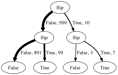
Each path from root to leaf of this tree represents a sequence of random choices made in evaluating the above program (the first flip for breast-cancer, the second for positive-mammogram), with the number of traversals and the sampled value labeling each edge. (Because this is 1000 random samples, the number are close (but not exactly) those in the Gigerenzer, et al, story.) Selecting just the 106 hypothetical cases of women with a positive mammogram, and computing the fraction of those who also have breast cancer (7/106), corresponds exactly to rejection-query. Thus, we have used the causal representation in the above church program to manufacture frequencies which can be used to arrive at the inference that relatively few women with positive mammograms actually have breast cancer.
Yet unlike the rejection sampler people are quite bad at reasoning in this scenario. Why? One answer is that people don’t represent their knowledge in quite the form of this simple church program. Indeed, Krynski & Tenenbaum (2007) have argued that human statistical judgment is fundamentally based on conditioning more explicit causal models: they suggested that “base rate neglect” and other judgment errors may occur when people are given statistical information that cannot be easily mapped to the parameters of the causal models they intuitively adopt to describe the situation. In the above example, they suggested that the notion of a false alarm rate is not intuitive to many people—particularly when the false alarm rate is ten times higher than the base rate of the disease that the test is intended to diagnose! They showed that “base rate neglect” could be eliminated by reformulating the breast cancer problem in terms of more intuitive causal models. For example, consider their version of the breast cancer problem (the exact numbers and wording differed slightly):
1% of women at age 40 who participate in a routine screening will have breast cancer. Of those with breast cancer, 80% will receive a positive mammogram. 20% of women at age 40 who participate in a routine screening will have a benign cyst. Of those with a benign cyst, 50% will receive a positive mammogram due to unusually dense tissue of the cyst. All others will receive a negative mammogram. Suppose that a woman in this age group has a positive mammography in a routine screening. What is the probability that she actually has breast cancer?
This question is easy for people to answer—empirically, just as easy as the frequency-based formulation given above. We may conjecture this is because the relevant frequencies can be computed from a simple query on the following more intuitive causal model:
(define samples
 (mh-query 100 100
   (define breast-cancer (flip 0.01))
   (define benign-cyst (flip 0.2))

   (define positive-mammogram (or (and breast-cancer (flip 0.8)) (and benign-cyst (flip 0.5))))

   breast-cancer

   positive-mammogram
 )
)
(hist samples "breast cancer")
Because this causal model—this Church program—is more intuitive to people, they can imagine the appropriate situations, despite having been given percentages rather than frequencies. What makes this causal model more intuitive than the one above with an explicitly specified false alarm rate? Essentially we have replaced probabilistic dependencies on the “non-occurrence” of events (e.g., the dependence of a positive mammogram on not having breast cancer) with dependencies on explicitly specified alternative causes for observed effects (e.g., the dependence of a positive mammogram on having a benign cyst).
A causal model framed in this way can scale up to significantly more complex situations. Recall our more elaborate medical diagnosis network from the previous section, which was also framed in this way using noisy-logical functions to describe the dependence of symptoms on disease:
(define samples
  (mh-query 1000 100
    (define lung-cancer (flip 0.01))
    (define TB (flip 0.005))
    (define cold (flip 0.2))
    (define stomach-flu (flip 0.1))
    (define other (flip 0.1))

    (define cough (or (and cold (flip 0.5)) (and lung-cancer (flip 0.3)) (and TB (flip 0.7)) (and other (flip 0.01))))
    (define fever (or (and cold (flip 0.3)) (and stomach-flu (flip 0.5)) (and TB (flip 0.2)) (and other (flip 0.01))))
    (define chest-pain (or (and lung-cancer (flip 0.4)) (and TB (flip 0.5)) (and other( flip 0.01))))
    (define shortness-of-breath (or (and lung-cancer (flip 0.4)) (and TB (flip 0.5)) (and other (flip 0.01))))

    (list lung-cancer TB)

    (and cough fever chest-pain shortness-of-breath)

  )
)
(hist samples "Joint inferences for lung cancer and TB")
You can use this model to infer conditional probabilities for any subset of diseases conditioned on any pattern of symptoms. Try varying the symptoms in the conditioning set or the diseases in the query, and see how the model’s inferences compare with your intuitions. For example, what happens to inferences about lung cancer and TB in the above model if you remove chest pain and shortness of breath as symptoms? (Why? Consider the alternative explanations.) More generally, we can condition on any set of events – any combination of symptoms and diseases – and query any others. We can also condition on the negation of an event using (not ...): e.g., how does the probability of lung cancer (versus TB) change if we observe that the patient does not have a fever, does not have a cough, or does not have either symptom?
A Church program thus effectively encodes the answers to a very large number of possible questions in a very compact form, where each question has the form, “Suppose we observe X, what can we infer about Y?”. In the program above, there are \(3^9=19683\) possible simple conditioners (possible X’s) corresponding to conjunctions of events or their negations (because the program has 9 stochastic Boolean-valued functions, each of which can be observed true, observed false, or not observed). Then for each of those X’s there are a roughly comparable number of Y’s, corresponding to all the possible conjunctions of variables that can be in the query set Y, making the total number of simple questions encoded on the order of 100 million. In fact, as we will see below when we describe complex queries, the true number of possible questions encoded in just a short Church program like this one is very much larger than that; usually the set is infinite. With query we can in principle compute the answer to every one of these questions. We are beginning to see the sense in which probabilistic programming provides the foundations for constructing a language of thought, as described in the Introduction: a finite system of knowledge that compactly and efficiently supports an infinite number of inference and decision tasks.
Expressing our knowledge as a probabilistic program of this form also makes it easy to add in new relevant knowledge we may acquire, without altering or interfering with what we already know. For instance, suppose we decide to consider behavioral and demographic factors that might contribute causally to whether a patient has a given disease:
(define samples
  (mh-query 1000 100
    (define works-in-hospital (flip 0.01))
    (define smokes (flip 0.2))

    (define lung-cancer (or (flip 0.01) (and smokes (flip 0.02))))
    (define TB (or (flip 0.005) (and works-in-hospital (flip 0.01))))
    (define cold (or (flip 0.2) (and works-in-hospital (flip 0.25))))
    (define stomach-flu (flip 0.1))
    (define other (flip 0.1))

    (define cough (or (and cold (flip 0.5)) (and lung-cancer (flip 0.3)) (and TB (flip 0.7)) (and other (flip 0.01))))
    (define fever (or (and cold (flip 0.3)) (and stomach-flu (flip 0.5)) (and TB (flip 0.2)) (and other (flip 0.01))))
    (define chest-pain (or (and lung-cancer (flip 0.4)) (and TB (flip 0.5)) (and other( flip 0.01))))
    (define shortness-of-breath (or (and lung-cancer (flip 0.4)) (and TB (flip 0.5)) (and other (flip 0.01))))

   (list lung-cancer TB)

   (and cough chest-pain shortness-of-breath)

  )
)
(hist samples "Joint inferences for lung cancer and TB")
Under this model, a patient with coughing, chest pain and shortness of breath is likely to have either lung cancer or TB. Modify the above code to see how these conditional inferences shift if you also know that the patient smokes or works in a hospital (where they could be exposed to various infections, including many worse infections than the typical person encounters). More generally, the causal structure of knowledge representation in a probabilistic program allows us to model intuitive theories that can grow in complexity continually over a lifetime, adding new knowledge without bound.
Exercises
Conditioning and prior manipulation: In the earlier Medical Diagnosis section we suggested understanding the patterns of symptoms for a particular disease by changing the prior probability of the disease such that it is always true.
For this example, does this procedure give the same answers as using
queryto condition on the disease being true?Why would this procedure give different answers than conditioning for more general hypotheticals? Construct an example where these are different. Then translate this into a Church model and show that manipulating the prior gives different answers than manipulating the observation. Hint: think about changing the prior versus observing a variable that has a causal parent.
Computing marginals: Use the rules for computing probabilities to compute the marginal distribution on return values from these Church programs.
(rejection-query
  (define a (flip))
  (define b (flip))
  a
  (or a b))
(rejection-query (define nice (mem (lambda (person) (flip 0.7)))) (define (smiles person) (if (nice person) (flip 0.8) (flip 0.5))) (nice 'alice) (and (smiles 'alice) (smiles 'bob) (smiles 'alice)))Extending the smiles model:
Describe (using ordinary English) what the second Church program above means.
Write a version of the model that captures these two intuitions: (1) people are more likely to smile if they want something and (2) nice people are less likely to want something.
Given your extended model, how would you ask whether someone wants something from you, given that they are smiling and have rarely smiled before? In your answer, show the Church query and a histogram of the answers – in what ways do these answers make intuitive sense or fail to?
Casino game. Consider the following game. A machine randomly gives Bob a letter of the alphabet; it gives a, e, i, o, u, y (the vowels) with probability 0.01 each and the remaining letters (i.e., the consonants) with probability 0.047 each. The probability that Bob wins depends on which letter he got. Letting \(h\) denote the letter and letting \(Q(h)\) denote the numeric position of that letter (e.g., \(Q(\text{a}) = 1, Q(\text{b}) = 2\), and so on), the probability of winning is \(1/Q(h)^2\). Suppose that we observe Bob winning but we don’t know what letter he got. How can we use the observation that he won to update our beliefs about which letter he got? Let’s express this formally. Before we begin, a bit of terminology: the set of letters that Bob could have gotten, \(\{a, b, c, d, ..., y, z\}\), is called the hypothesis space – it’s our set of hypotheses about the letter.
- In English, what does the posterior probability \(p(h \mid \text{win})\) represent?
- Manually compute \(p(h \mid \text{win})\) for each hypothesis (Excel or something like it is helpful here). Remember to normalize - make sure that summing all your \(p(h \mid \text{win})\) values gives you 1.
Now, we’re going to write this model in Church using
enumeration-query. Here is some starter code for you:;; define some variables and utility functions (define letters '(a b c d e f g h i j k l m n o p q r s t u v w x y z) ) (define (vowel? letter) (if (member letter '(a e i o u y)) #t #f)) (define letter-probabilities (map (lambda (letter) (if (vowel? letter) 0.01 0.047)) letters)) (define (my-list-index needle haystack counter) (if (null? haystack) 'error (if (equal? needle (first haystack)) counter (my-list-index needle (rest haystack) (+ 1 counter))))) (define (get-position letter) (my-list-index letter letters 1)) ;; actually compute p(h | win) (define distribution (enumeration-query (define my-letter (multinomial letters letter-probabilities)) (define my-position (get-position my-letter)) (define my-win-probability (/ 1.0 (* my-position my-position))) (define win? ...) ;; query ... ;; condition ... )) (barplot distribution)Note that you don’t use
historrepeathere. Withenumeration-query, function calls directly correspond to distributions (whereas withrejection-queryormh-query, function calls correspond only to samples and you have to build the data for histograms manually). If you have a distribution, you callbarplot.What does the
my-list-indexfunction do? What would happen if you ran(my-list-index 'mango '(apple banana) 1)?What does the
multinomialfunction do? Usemultinomialto express this distribution:x P(x) red 0.5 blue 0.05 green 0.4 black 0.05 (define x ...)Fill in the
...’s in the code to compute \(p(h \mid \text{win})\). Include a screenshot of the resulting graph. What letter has the highest posterior probability? In English, what does it mean that this letter has the highest posterior? Make sure that your Church answers and hand-computed answers agree – note that this demonstrates the equivalence between the program view of conditional probability and the distributional view.Which is higher, \(p(\text{vowel} \mid \text{win})\) or \(p(\text{consonant} \mid \text{win})\)? Answer this using the Church code you wrote (hint: use the
vowel?function)What difference do you see between your code and the mathematical notation? What are the advantages and disadvantages of each? Which do you prefer?
References
Gerstenberg2012Gerstenberg, T., & Goodman, N. D. (2012). Ping pong in Church: Productive use of concepts in human probabilistic inference. In Proceedings of the 34th Annual Conference of the Cognitive Science Society. Retrieved from http://www.stanford.edu/~ngoodman/papers/GerstenbergGoodman2012.pdf
Gigerenzer1995Gigerenzer, G., & Hoffrage, U. (1995). How to improve Bayesian reasoning without instruction: Frequency formats. Psychological Review, 102(4), 684.
Krynski, T. R., & Tenenbaum, J. B. (2007). The role of causality in judgment under uncertainty. Journal of Experimental Psychology: General, 136(3), 430.
Tversky1974Tversky, A., & Kahneman, D. (1974). Judgment under uncertainty: Heuristics and biases. Science, 185(4157), 1124–1131.