4. Patterns of inference
Causal Dependence
Probabilistic programs encode knowledge about the world in the form of causal models, and it is useful to understand how their function relates to their structure by thinking about some of the intuitive properties of causal relations. Causal relations are local, modular, and directed. They are modular in the sense that any two arbitrary events in the world are most likely causally unrelated, or independent. If they are related, or dependent, the relation is only very weak and liable to be ignored in our mental models. Causal structure is local in the sense that many events that are related are not related directly: They are connected only through causal chains of several steps, a series of intermediate and more local dependencies. And the basic dependencies are directed: when we say that A causes B, it means something different than saying that B causes A.The causal influence flows only one way along a causal relation—we expect that manipulating the cause will change the effect, but not vice versa—but information can flow both ways—learning about either event will give us information about the other.
Let’s examine this notion of “causal dependence” a little more carefully. What does it mean to believe that A depends causally on B? Viewing cognition through the lens of probabilistic programs, the most basic notions of causal dependence are in terms of the structure of the program and the flow of evaluation (or “control”) in its execution. We say that expression A causally depends on expression B if it is necessary to evaluate B in order to evaluate A. (More precisely, expression A depends on expression B if it is ever necessary to evaluate B in order to evaluate A.) For instance, in this program A depends on B but not on C (the final expression depends on both A and C):
(define C (flip))
(define B (flip))
(define A (if B (flip 0.1) (flip 0.4)))
(or A C)
Note that causal dependence order is weaker than a notion of ordering in time—one expression might happen to be evaluated before another in time (for instance C before A), but without the second expression requiring the first. (This notion of causal dependence is related to the notion of flow dependence in the programming language literature.)
For example, consider a simpler variant of our medical diagnosis scenario:
(define samples
  (mh-query
   200 100

   (define smokes (flip 0.2))

   (define lung-disease (or (flip 0.001) (and smokes (flip 0.1))))
   (define cold (flip 0.02))

   (define cough (or (and cold (flip 0.5)) (and lung-disease (flip 0.5)) (flip 0.01)))
   (define fever (or (and cold (flip 0.3)) (flip 0.01)))
   (define chest-pain (or (and lung-disease (flip 0.2)) (flip 0.01)))
   (define shortness-of-breath (or (and lung-disease (flip 0.2)) (flip 0.01)))

   (list cold lung-disease)

   cough))

(hist (map first samples) "cold")
(hist (map second samples) "lung-disease")
(hist samples "cold, lung-disease")
Here, cough depends causally on both lung-disease and cold, while fever depends causally on cold but not lung-disease. We can see that cough depends causally on smokes but only indirectly: although cough does not call smokes directly, in order to evaluate whether a patient coughs, we first have to evaluate the expression lung-disease that must itself evaluate smokes.
We haven’t made the notion of “direct” causal dependence precise: do we want to say that cough depends directly on cold, or only directly on the expression (or (and cold (flip 0.5)) ...? This can be resolved in several ways that all result in similar intuitions. For instance, we could first re-write the program into a form where each intermediate expression is named (called A-normal form) and then say direct dependence is when one expression immediately includes the name of another.
There are several special situations that are worth mentioning. In some cases, whether expression A requires expression B will depend on the value of some third expression C. For example, here is a particular way of writing a noisy-AND relationship:
(define C (flip))
(define B (flip))
(define A (if C (if B (flip 0.85) false) false))
A
A always requires C, but only evaluates B if C returns true. Under the above definition of causal dependence A depends on B (as well as C). However, one could imagine a more fine-grained notion of causal dependence that would be useful here: we could say that A depends causally on B only in certain contexts (just those where C happens to return true and thus A calls B).
Another nuance is that an expression that occurs inside a function body may get evaluated several times in a program execution. In such cases it is useful to speak of causal dependence between specific evaluations of two expressions. (However, note that if a specific evaluation of A depends on a specific evaluation of B, then any other specific evaluation of A will depend on some specific evaluation of B. Why?)
Detecting Dependence Through Intervention
The causal dependence structure is not always immediately clear from examining a program, particularly where there are complex functions calls. Another way to detect (or according to some philosophers, such as Jim Woodward, to define) causal dependence is more operational, in terms of “difference making”: If we manipulate A, does B tend to change? By manipulate here we don’t mean an assumption in the sense of query. Instead we mean actually edit, or intervene on, the program in order to make an expression have a particular value independent of its (former) causes. If setting A to different values in this way changes the distribution of values of B, then B causally depends on A. This method is known in the causal Bayesian network literature as the “do operator” or graph surgery (Pearl, 1988). It is also the basis for interesting theories of counterfactual reasoning by Pearl and colleagues (Halpern, Hitchcock and others).
For example, this code represents whether a patient is likely to have a cold or a cough a priori, conditioned on no observations:
(define (sample)
  (define smokes (flip 0.2))

  (define lung-disease (or (flip 0.001) (and smokes (flip 0.1))))
  (define cold (flip 0.02))

  (define cough (or (and cold (flip 0.5)) (and lung-disease (flip 0.5)) (flip 0.01)))
  (define fever (or (and cold (flip 0.3)) (flip 0.01)))
  (define chest-pain (or (and lung-disease (flip 0.2)) (flip 0.01)))
  (define shortness-of-breath (or (and lung-disease (flip 0.2)) (flip 0.01)))

  (list cough cold))

(define samples (repeat 200 sample))

(hist (map first samples) "cough")
(hist (map second samples) "cold")
Imagine we now give our hypothetical patient a cold—for example, by exposing him to a strong cocktail of cold viruses. We should not model this as an observation (conditioning on having a cold using query), because we have taken direct action to change the normal causal structure. Instead we implement intervention by directly editing the program: first do (define cold true), then do (define cold false):
(define (sample)
  (define smokes (flip 0.2))

  (define lung-disease (or (flip 0.001) (and smokes (flip 0.1))))
  (define cold true) ;we intervene to make cold true.

  (define cough (or (and cold (flip 0.5)) (and lung-disease (flip 0.5)) (flip 0.01)))
  (define fever (or (and cold (flip 0.3)) (flip 0.01)))
  (define chest-pain (or (and lung-disease (flip 0.2)) (flip 0.01)))
  (define shortness-of-breath (or (and lung-disease (flip 0.2)) (flip 0.01)))

  (list cough cold))

(define samples (repeat 200 sample))

(hist (map first samples) "cough")
(hist (map second samples) "cold")
You should see that the distribution on cough changes: coughing becomes more likely if we know that a patient has been given a cold by external intervention. But the reverse is not true. Try forcing the patient to have a cough (e.g., with some unusual drug or by exposure to some cough-inducing dust) by writing (define cough true): the distribution on cold is unaffected. We have captured a familiar fact: treating the symptoms of a disease directly doesn’t cure the disease (taking cough medicine doesn’t make your cold go away), but treating the disease does relieve the symptoms.
Verify in the program above that the method of manipulation works also to identify causal relations that are only indirect: for example, force a patient to smoke and show that it increases their probability of coughing, but not vice versa. If we are given a program representing a causal model, and the model is simple enough, it is straightforward to read off causal dependencies from the structure of the program. However, the notion of causation as difference-making may be easier to compute in much larger, more complex models—and it does not require an analysis of the program code. As long as we can modify (or imagine modifying) the definitions in the program and can run the resulting model, we can compute whether two events or functions are causally related by the difference-making criterion.
Statistical Dependence
One often hears the warning, “correlation does not imply causation”. By “correlation” we mean a different kind of dependence between events or functions—statistical dependence. We say that A and B are statistically dependent, if learning information about A tells us something about B, and vice versa. In the language of Church: using query to make an assumption about A changes the value expected for B. Statistical dependence is a symmetric relation between events referring to how information flows between them when we observe or reason about them. (If using query to condition on A changes B, then conditioning on B also changes A. Why?) The fact that we need to be warned against confusing statistical and causal dependence suggests they are related, and indeed, they are. In general, if A causes B, then A and B will be statistically dependent. (One might even say the two notions are “causally related”, in the sense that causal dependencies give rise to statistical dependencies.)
Diagnosing statistical dependence using query is similar to diagnosing causal dependence through intervention. We query on the target variable, here A, conditioning on various values of the possible statistical dependent, here B:
(define (samples B-val)
  (mh-query
   100 10
   (define C (flip))
   (define B (flip))
   (define A (if B (flip 0.1) (flip 0.4)))
   A
   (eq? B B-val)))

(hist (samples true) "A if B is true.")
(hist (samples false) "A if B is false.")
Because the two distributions on A (when we have different information about B) are different, we can conclude that A statistically depends on B. Do the same procedure for testing if B statistically depends on A. How is this similar (and different) from the causal dependence between these two? As an exercise, make a version of the above medical example to test the statistical dependence between cough and cold. Verify that statistical dependence holds symmetrically for events that are connected by an indirect causal chain, such as smokes and coughs.
Correlation is not just a symmetrized version of causality. Two events may be statistically dependent even if there is no causal chain running between them, as long as they have a common cause (direct or indirect). That is, two expressions in a Church program can be statistically dependent if one calls the other, directly or indirectly, or if they both at some point in their evaluation histories refer to some other expression (a “common cause”). Here is an example of statistical dependence generated by a common cause:
(define (samples B-val)
  (mh-query
   100 10
   (define C (flip))
   (define B (if C (flip 0.5) (flip 0.9)))
   (define A (if C (flip 0.1) (flip 0.4)))
   A
   (eq? B B-val)))

(hist (samples true) "A if B is true.")
(hist (samples false) "A if B is false.")
Situations like this are extremely common. In the medical example above, cough and fever are not causally dependent but they are statistically dependent, because they both depend on cold; likewise for chest-pain and shortness-of-breath which both depend on lung-disease. Here we can read off these facts from the program definitions, but more generally all of these relations can be diagnosed by reasoning using query.
Successful learning and reasoning with causal models typically depends on exploiting the close coupling between causation and correlation. Causal relations are typically unobservable, while correlations are observable from data. Noticing patterns of correlation is thus often the beginning of causal learning, or discovering what causes what. On the other hand, with a causal model already in place, reasoning about the statistical dependencies implied by the model allows us to predict many aspects of the world not directly observed from those aspects we do observe.
Graphical Notations for Dependence
Graphical models are an extremely important idea in modern machine learning: a graphical diagram is used to represent the direct dependence structure between random choices in a probabilistic model. A special case are Bayesian networks, in which there is a node for each random variable (and expression in our terms) and a link between two nodes if there is a direct conditional dependence between them (a direct causal dependence in our terms). The sets of nodes and links define a directed acyclic graph (hence the term graphical model), a data structure over which many efficient algorithms can be defined. Each node has a conditional probability table (CPT), which represents the conditional probability distribution of that node, given its parents. The joint probability distribution over random variables is given by the product of the conditional distributions for each variable in the graph.
The figure below defines a Bayesian network for the medical diagnosis example. The graph contains a node for each define statement in our church program, with links to that node from each variable that appears in the assignment expression. There is a probability table (“CPT”) for each node, with a column for each value of the variable, and a row for each combination of values for its parents in the graph.
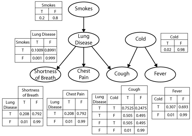
Simple generative models will have a corresponding graphical model that captures all of the dependencies (and independencies) of the model, without capturing the precise form of these functions. For example, while the graphical model shown above faithfully represents the probability distribution encoded by the church program, it captures the noisy-OR form of the causal dependencies only implicitly. As a result, the CPTs provide a less compact representation of the conditional probabilities than the church model. For instance, the CPT for cough specifies 4 parameters – one for each pair of values of lung-disease and cold (the second entry in each row is determined by the constraint that the conditional distribution of cough must sum to 1). In contrast, the define statement for cough in church specifies only 3 parameters: the base rate of cough, and the strength with which lung-disease and cold cause cough. This difference becomes more pronounced for noisy-OR relations with many causes – the size of the CPT for a node will be exponential in the number of parents, while the number of terms in the noisy-OR expression in church for that node will be linear in the number of causal dependencies (why?). As we will see, this has important implications for the ability to learn the values of the parameters from data.
More complicated generative models, which can be expressed as probabilistic programs, often don’t have such a graphical model (or rather they have many approximations, none of which captures all independencies). Recursive models generally give rise to such ambiguous (or loopy) Bayes nets.
From A Priori Dependence to Conditional Dependence
The relationships between causal structure and statistical dependence become particularly interesting and subtle when we look at the effects of additional observations or assumptions. Events that are statistically dependent a priori (sometimes called marginally dependent) may become independent when we condition on some other observation; this is called screening off, or sometimes context-specific independence. Also, events that are statistically independent a priori (marginally independent) may become dependent when we condition on other observations; this is known as explaining away. The dynamics of screening off and explaining away are extremely important for understanding patterns of inference—reasoning and learning—in probabilistic models.
Screening off
Screening off refers to a pattern of statistical inference that is quite common in both scientific and intuitive reasoning. If the statistical dependence between two events A and B is only indirect, mediated strictly by one or more other events C, then conditioning on (observing) C should render A and B statistically independent. This can occur if A and B are connected by one or more causal chains, and all such chains run through the set of events C, or if C comprises one or more common causes of A and B.
For instance, let’s look again at our common cause example, this time assuming that we already know the value of C:
(define (samples B-val)
  (mh-query
   100 10
   (define C (flip))
   (define B (if C (flip 0.5) (flip 0.9)))
   (define A (if C (flip 0.1) (flip 0.4)))
   A
   (and C (eq? B B-val))))

(hist (samples true) "A if B is true.")
(hist (samples false) "A if B is false.")
We see that A an B are statistically independent given knowledge of C. (Note: it can be tricky to diagnose statistical independence from samples, such as returned by mh-query, since natural variation due to random sampling can look like differences between conditions.)
Screening off is a purely statistical phenomenon. For example, consider the the causal chain model, where A directly causes C, which in turn directly causes B. Here, when we observe C – the event that mediates an indirect causal relation between A and B – A and B are still causally dependent in our model of the world: it is just our beliefs about the states of A and B that become uncorrelated. There is also an analogous causal phenomenon. If we can actually manipulate or intervene on the causal system, and set the value of C to some known value, then A and B become both statistically and causally independent (by intervening on C, we break the causal link between A and C).
Explaining away
“Explaining away” (Pearl, 1988) refers to a complementary pattern of statistical inference which is somewhat more subtle than screening off. If two events A and B are statistically (and hence causally) independent, but they are both causes of one or more other events C, then conditioning on (observing) C can render A and B statistically dependent. Here is an example where A and B have a common effect:
(define (samples B-val)
  (mh-query
   100 10
   (define A (flip))
   (define B (flip))
   (define C (if (or A B) (flip 0.9) (flip 0.2)))
    A
   (and C (eq? B B-val))))

(hist (samples true) "A if B is true.")
(hist (samples false) "A if B is false.")
As with screening off, we only induce statistical dependence from learning about C, not causal dependence: when we observe C, A and B remain causally independent in our model of the world; it is our beliefs about A and B that become correlated.
We can express the general phenomenon of explaining away with the following schematic Church query:
(query
  (define a ...)
  (define b ...)
  ...
  (define data (... a... b...))

  b

  (and (equal? data some-value) (equal? a some-other-value)))
We have defined two independent variables a and b both of which are used to define the value of our data. If we condition on the data and a the posterior distribution on b will now be dependent on a: observing additional information about a changes our conclusions about b.
The most typical pattern of explaining away we see in causal reasoning is a kind of anti-correlation: the probabilities of two possible causes for the same effect increase when the effect is observed, but they are conditionally anti-correlated, so that observing additional evidence in favor of one cause should lower our degree of belief in the other cause. However, the coupling induced by conditioning on common effects depends on the nature of the interaction between the causes, it is not always an anti-correlation. Explaining away takes the form of an anti-correlation when the causes interact in a roughly disjunctive or additive form: the effect tends to happen if any cause happens; or the effect happens if the sum of some continuous influences exceeds a threshold. The following simple mathematical examples show this and other patterns.
Suppose we condition on observing the sum of two integers drawn uniformly from 0 to 9:
(define (take-sample)
  (rejection-query
    (define A (random-integer 10))
    (define B (random-integer 10))

    (pair A B)

    (equal? (+ A B) 9)))

(define samples (repeat 500 take-sample))

(scatter samples "A and B, conditioned on A + B = 9")
(hist samples "A, B")
This gives perfect anti-correlation in conditional inferences for A and B. But suppose we instead condition on observing that A and B are equal:
(define (take-sample)
  (rejection-query
    (define A (random-integer 10))
    (define B (random-integer 10))

    (pair A B)

    (equal? A B)))

(define samples (repeat 500 take-sample))

(scatter samples "A and B, conditioned on A = B")
(hist samples "A, B")
Now, of course, A and B go from being independent a priori to being perfectly correlated in the conditional distribution. Try out these other conditioners to see other possible patterns of conditional dependence for a priori independent functions:
(< (abs (- A B)) 2)(and (>= (+ A B) 9) (<= (+ A B) 11))(equal? 3 (abs (- A B)))(equal? 3 (mod (- A B) 10))(equal? (mod A 2) (mod B 2))(equal? (mod A 5) (mod B 5))
Non-monotonic Reasoning
One reason explaining away is an important phenomenon in probabilistic inference is that it is an example of non-monotonic reasoning. In formal logic, a theory is said to be monotonic if adding an assumption (or formula) to the theory never reduces the set of conclusions that can be drawn. Most traditional logics (e.g. First Order) are monotonic, but human reasoning does not seem to be. For instance, if I tell you that Tweety is a bird, you conclude that he can fly; if I now tell you that Tweety is an ostrich you retract the conclusion that he can fly. Over the years many non-monotonic logics have been introduced to model aspects of human reasoning. One of the first reasons that probabilistic reasoning with Bayesian networks was recognized as important for AI was that it could perspicuously capture these patterns of reasoning (see for instance Pearl, 1988).
Another way to think about monotonicity is by considering the trajectory of our belief in a specific proposition, as we gain additional relevant information. In traditional logic, there are only three states of belief: true, false, and unknown (when neither a proposition nor its negation can be proven). As we learn more about the world, maintaining logical consistency requires that our belief in any proposition only move from unknown to true or false. That is our “confidence” in any conclusion only increases (and only does so in one giant leap from unknown to true or false).
In a probabilistic approach, by contrast, belief comes in a whole spectrum of degrees. We can think of confidence as a measure of how far our beliefs are from a uniform distribution—how close to the extremes of 0 or 1. In probabilistic inference, unlike in traditional logic, our confidence in a proposition can both increase and decrease. Even fairly simple probabilistic models can induce complex explaining-away dynamics that lead our degree of belief in a proposition to reverse directions multiple times as the conditioning set expands.
Example: Medical Diagnosis
The medical scenario is a great model to explore screening off and explaining away. In this model smokes is statistically dependent on several symptoms—cough, chest-pain, and shortness-of-breath—due to a causal chain between them mediated by lung-disease. We can see this easily by conditioning on these symptoms and querying smokes:
(define samples
  (mh-query 200 100
    (define smokes (flip 0.2))

    (define lung-disease (or (flip 0.001) (and smokes (flip 0.1))))
    (define cold (flip 0.02))

    (define cough (or (and cold (flip 0.5)) (and lung-disease (flip 0.5)) (flip 0.001)))
    (define fever (or (and cold (flip 0.3)) (flip 0.01)))
    (define chest-pain (or (and lung-disease (flip 0.2)) (flip 0.01)))
    (define shortness-of-breath (or (and lung-disease (flip 0.2)) (flip 0.01)))

     smokes

     (and cough chest-pain shortness-of-breath)
  )
)
(hist samples "smokes")
The conditional probability of smokes is much higher than the base rate, 0.2, because observing all these symptoms gives strong evidence for smoking. See how much evidence the different symptoms contribute by dropping them out of the conditioning set. For instance, condition the above query on (and cough chest-pain), or just cough; you should observe the probability of smokes decrease as fewer symptoms are observed.
Now, suppose we condition also on knowledge about the function that mediates these causal links: lung-disease. Is there still an informational dependence between these various symptoms and smokes? In the query below, try adding and removing various symptoms (cough, chest-pain, shortness-of-breath) but maintaining the observation lung-disease:
(define samples
  (mh-query 500 100
    (define smokes (flip 0.2))

    (define lung-disease (or (flip 0.001) (and smokes (flip 0.1))))
    (define cold (flip 0.02))

    (define cough (or (and cold (flip 0.5)) (and lung-disease (flip 0.5)) (flip 0.001)))
    (define fever (or (and cold (flip 0.3)) (flip 0.01)))
    (define chest-pain (or (and lung-disease (flip 0.2)) (flip 0.01)))
    (define shortness-of-breath (or (and lung-disease (flip 0.2)) (flip 0.01)))

     smokes

     (and lung-disease
          (and cough chest-pain shortness-of-breath)
      )
  )
)
(hist samples "smokes")
You should see an effect of whether the patient has lung disease on conditional inferences about smoking—a person is judged to be substantially more likely to be a smoker if they have lung disease than otherwise—but there is no separate effects of chest pain, shortness of breath or cough, over and above the evidence provided by knowing whether the patient has lung-disease. We say that the intermediate variable lung disease screens off the root cause (smoking) from the more distant effects (coughing, chest pain and shortness of breath).
Here is a concrete example of explaining away in our medical scenario. Having a cold and having lung disease are a priori independent both causally and statistically. But because they are both causes of coughing if we observe cough then cold and lung-disease become statistically dependent. That is, learning something about whether a patient has cold or lung-disease will, in the presence of their common effect cough, convey information about the other condition. We say that cold and lung-cancer are marginally (or a priori) independent, but conditionally dependent given cough.
To illustrate, observe how the probabilities of cold and lung-disease change when we observe cough is true:
(define samples
  (mh-query 500 100
    (define smokes (flip 0.2))

    (define lung-disease (or (flip 0.001) (and smokes (flip 0.1))))
    (define cold (flip 0.02))

    (define cough (or (and cold (flip 0.5)) (and lung-disease (flip 0.5)) (flip 0.001)))
    (define fever (or (and cold (flip 0.3)) (flip 0.01)))
    (define chest-pain (or (and lung-disease (flip 0.2)) (flip 0.01)))
    (define shortness-of-breath (or (and lung-disease (flip 0.2)) (flip 0.01)))

   (list cold lung-disease)

   cough))

(hist (map first samples) "cold")
(hist (map second samples) "lung-disease")
(hist samples "cold, lung-disease")
Both cold and lung disease are now far more likely that their baseline probability: the probability of having a cold increases from 2% to around 50%; the probability of having lung disease also increases from 1 in a 1000 to around 50%.
Now suppose we learn that the patient does not have a cold.
(define samples
  (mh-query 500 100
    (define smokes (flip 0.2))

    (define lung-disease (or (flip 0.001) (and smokes (flip 0.1))))
    (define cold (flip 0.02))

    (define cough (or (and cold (flip 0.5)) (and lung-disease (flip 0.5)) (flip 0.001)))
    (define fever (or (and cold (flip 0.3)) (flip 0.01)))
    (define chest-pain (or (and lung-disease (flip 0.2)) (flip 0.01)))
    (define shortness-of-breath (or (and lung-disease (flip 0.2)) (flip 0.01)))

   (list cold lung-disease)

   (and cough (not cold))))

(hist (map first samples) "cold")
(hist (map second samples) "lung-disease")
(hist samples "cold, lung-disease")
The probability of having lung disease increases dramatically. If instead we had observed that the patient does have a cold, the probability of lung cancer returns to its very low base rate of 1 in a 1000.
(define samples
  (mh-query 500 100
    (define smokes (flip 0.2))

    (define lung-disease (or (flip 0.001) (and smokes (flip 0.1))))
    (define cold (flip 0.02))

    (define cough (or (and cold (flip 0.5)) (and lung-disease (flip 0.5)) (flip 0.001)))
    (define fever (or (and cold (flip 0.3)) (flip 0.01)))
    (define chest-pain (or (and lung-disease (flip 0.2)) (flip 0.01)))
    (define shortness-of-breath (or (and lung-disease (flip 0.2)) (flip 0.01)))

   (list cold lung-disease)

   (and cough cold)))

(hist (map first samples) "cold")
(hist (map second samples) "lung-disease")
(hist samples "cold, lung-disease")
This is the conditional statistical dependence between lung disease and cold, given cough: Learning that the patient does in fact have a cold “explains away” the observed cough, so the alternative of lung disease decreases to a much lower value — roughly back to its 1 in a 1000 rate in the general population. If on the other hand, we had learned that the patient does not have a cold, so the most likely alternative to lung disease is not in fact available to “explain away” the observed cough, that raises the conditional probability of lung disease dramatically. As an exercise, check that if we remove the observation of coughing, the observation of having a cold or not has no influence on our belief about lung disease; this effect is purely conditional on the observation of a common effect of these two causes.
Explaining away effects can be more indirect. Instead of observing the truth value of cold, a direct alternative cause of cough, we might simply observe another symptom that provides evidence for cold, such as fever. Compare these conditioners with the above church program to see an “explaining away” conditional dependence in belief between fever and lung-disease. Replace (and smokes chest-pain cough) with (and smokes chest-pain cough fever) or (and smokes chest-pain cough (not fever)). In this case, finding out that the patient either does or does not have a fever makes a crucial difference in whether we think that the patient has lung disease… even though fever itself is not at all diagnostic of lung disease, and there is no causal connection between them.
Example: Trait Attribution
People often have to make inferences about entities and their interactions. Such problems tend to have dense relations between the entities, leading to very challenging explaining away problems. Inference is computationally difficult in these situations but the inferences come very naturally to people, suggesting these are important problems that our brains have specialized somewhat to solve (or perhaps that they have evolved general solutions to these tough inferences).
A familiar example comes from reasoning about the causes of students’ success and failure in the classroom. Imagine yourself in the position of an interested outside observer—a parent, another teacher, a guidance counselor or college admissions officer—in thinking about these conditional inferences. If a student doesn’t pass an exam, what can you say about why he failed? Maybe he doesn’t do his homework, maybe the exam was unfair, or maybe he was just unlucky?
(define samples
  (mh-query 1000 10

   (define exam-fair (flip .8))
   (define does-homework (flip .8))

   (define pass? (flip (if exam-fair
                           (if does-homework 0.9 0.4)
                           (if does-homework 0.6 0.2))))

   (list does-homework exam-fair)

   (not pass?)))

(hist samples "Joint: Student Does Homework?, Exam Fair?")
(hist (map first samples) "Student Does Homework")
(hist (map second samples) "Exam Fair")
Now what if you have evidence from several students and several exams? We first re-write the above model to allow many students and exams:
(define samples
  (mh-query 1000 10

   (define exam-fair-prior .8)
   (define does-homework-prior .8)
   (define exam-fair? (mem (lambda (exam) (flip exam-fair-prior))))
   (define does-homework? (mem (lambda (student) (flip does-homework-prior))))

   (define (pass? student exam) (flip (if (exam-fair? exam)
                                          (if (does-homework? student) 0.9 0.4)
                                          (if (does-homework? student) 0.6 0.2))))

   (list (does-homework? 'bill) (exam-fair? 'exam1))

   (not (pass? 'bill 'exam1))))

(hist samples "Joint: Student Does Homework?, Exam Fair?")
(hist (map first samples) "Student Does Homework")
(hist (map second samples) "Exam Fair")
Initially we observe that Bill failed exam 1. A priori, we assume that most students do their homework and most exams are fair, but given this one observation it becomes somewhat likely that either the student didn’t study or the exam was unfair.
Notice that we have set the probabilities in the pass? function to be asymmetric: whether a student does homework has a greater influence on passing the test than whether the exam is fair. This in turns means that when inferring the cause of a failed exam, the model tends to attribute it to the person property (not doing homework) over the situation property (exam being unfair). This asymmetry is an example of the fundamental attribution bias (Ross, 1977): we tend to attribute outcomes to personal traits rather than situations. However there are many interacting tendencies (for instance the direction of this bias switches for members of some east-asian cultures). How could you extend the model to account for these interactions?
See how conditional inferences about Bill and exam 1 change as you add in more data about this student or this exam, or additional students and exams. Try using each of the below expressions as the condition for the above inference. Try to explain the different inferences that result at each stage. What does each new piece of the larger data set contribute to your intuition about Bill and exam 1?
(and (not (pass? 'bill 'exam1)) (not (pass? 'bill 'exam2)))

(and (not (pass? 'bill 'exam1))
          (not (pass? 'mary 'exam1))
          (not (pass? 'tim 'exam1)))

 (and (not (pass? 'bill 'exam1)) (not (pass? 'bill 'exam2))
       (not (pass? 'mary 'exam1))
       (not (pass? 'tim 'exam1)))

  (and (not (pass? 'bill 'exam1))
       (not (pass? 'mary 'exam1)) (pass? 'mary 'exam2) (pass? 'mary 'exam3) (pass? 'mary 'exam4) (pass? 'mary 'exam5)
       (not (pass? 'tim 'exam1)) (pass? 'tim 'exam2) (pass? 'tim 'exam3) (pass? 'tim 'exam4) (pass? 'tim 'exam5))

  (and (not (pass? 'bill 'exam1))
       (pass? 'mary 'exam1)
       (pass? 'tim 'exam1))

  (and (not (pass? 'bill 'exam1))
       (pass? 'mary 'exam1) (pass? 'mary 'exam2) (pass? 'mary 'exam3) (pass? 'mary 'exam4) (pass? 'mary 'exam5)
       (pass? 'tim 'exam1) (pass? 'tim 'exam2) (pass? 'tim 'exam3) (pass? 'tim 'exam4) (pass? 'tim 'exam5))

  (and (not (pass? 'bill 'exam1)) (not (pass? 'bill 'exam2))
       (pass? 'mary 'exam1) (pass? 'mary 'exam2) (pass? 'mary 'exam3) (pass? 'mary 'exam4) (pass? 'mary 'exam5)
       (pass? 'tim 'exam1) (pass? 'tim 'exam2) (pass? 'tim 'exam3) (pass? 'tim 'exam4) (pass? 'tim 'exam5))

  (and (not (pass? 'bill 'exam1)) (not (pass? 'bill 'exam2)) (pass? 'bill 'exam3) (pass? 'bill 'exam4) (pass? 'bill 'exam5)
       (not (pass? 'mary 'exam1)) (not (pass? 'mary 'exam2)) (not (pass? 'mary 'exam3)) (not (pass? 'mary 'exam4)) (not (pass? 'mary 'exam5))
       (not (pass? 'tim 'exam1)) (not (pass? 'tim 'exam2)) (not (pass? 'tim 'exam3)) (not (pass? 'tim 'exam4)) (not (pass? 'tim 'exam5)))
This example is inspired by the work of Harold Kelley (and many others) on causal attribution in social settings (Kelley, 1973). Kelley identified three important dimensions of variation in the evidence, which affect the attributions people make of the cause of an outcome. These three dimensions are: Persons—is the outcome consistent across different people in the situation?; Entities—is the outcome consistent for different entities in the situation?; Time—is the outcome consistent over different episodes? These dimensions map onto the different sets of evidence we have just seen—how?
Example: Of Blickets and Blocking
A number of researchers have explored children’s causal learning abilities by using the “blicket detector” (Gopnik & Sobel, 2000): a toy box that will light up when certain blocks, the blickets, are put on top of it. Children are shown a set of evidence and then asked which blocks are blickets. For instance, if block A makes the detector go off, it is probably a blicket. Ambiguous patterns are particularly interesting. Imagine that blocks A and B are put on the detector together, making the detector go off; it is likely that A is a blicket. Now B is put on the detector alone, making the detector go off; it is now less plausible that A is a blicket. This is called “backward blocking”, and it is an example of explaining away.
We can capture this set up with a model in which each block has a persistent “blicket-ness” property, and the causal power of the block to make the machine go off depends on its blicketness. Finally, the machine goes off if any of the blocks on it is a blicket (but noisily).
(define samples
  (mh-query 100 100

    (define blicket (mem (lambda (block) (flip 0.2))))
    (define (power block) (if (blicket block) 0.9 0.05))

    (define (machine blocks)
      (if (null? blocks)
          (flip 0.05)
          (or (flip (power (first blocks)))
              (machine (rest blocks)))))

    (blicket 'A)

    (machine (list 'A 'B))))

(hist samples "Is A a blicket?")
Try the backward blocking scenario described above. Sobel, Tenenbaum, & Gopnik (2004) tried this with children, finding that four year-olds perform similarly to the model: evidence that B is a blicket explains away the evidence that A and B made the detector go away.
A Case Study in Modularity: Visual Perception of Surface Lightness and Color
Visual perception is full of rich conditional inference phenomena, including both screening off and explaining away. Some very impressive demonstrations have been constructed using the perception of surface structure by mid-level vision researchers; see the work of Dan Kersten, David Knill, Ted Adelson, Bart Anderson, Ken Nakayama, among others. Most striking is when conditional inference appears to violate or alter the apparently “modular” structure of visual processing. Neuroscientists have developed an understanding of the primate visual system in which processing for different aspects of visual stimuli—color, shape, motion, stereo—appears to be at least somewhat localized in different brain regions. This view is consistent with findings by cognitive psychologists that at least in early vision, these different stimulus dimensions are not integrated but processed in a sequential, modular fashion. Yet vision is at heart about constructing a unified and coherent percept of a three-dimensional scene from the patterns of light falling on our retinas. That is, vision is causal inference on a grand scale. Its output is a rich description of the objects, surface properties and relations in the world that are not themselves directly grasped by the brain but that are the true causes of the input—low-level stimulation of the retinal. Solving this problem requires integration of many appearance features across an image, and this results in the potential for massive effects of explaining away and screening off.
In vision, the luminance of a surface depends on two factors, the illumination of the surface (how much light is hitting it) and its reflectance. The actual luminance is the product of the two factors. Thus luminance is inherently ambiguous. The visual system has to determine what proportion of the luminance is due to reflectance and what proportion is due to the illumination of the scene. This has led to a famous illusion known as the checker shadow illusion discovered by Ted Adelson.
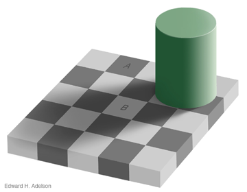
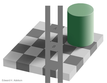
Despite appearances, in the image above both the square labeled A and the square labeled B are actually the same shade of gray. This can be seen in the figure below where they are connected by solid gray bars on either side.
The presence of the cylinder is providing evidence that the illumination of square B is actually less than that of square A (because it is expected to cast a shadow). Thus we perceive square B as having higher reflectance since its luminance is identical to square A and we believe there is less light hitting it. The following program implements a simple version of this scenario “before” we see the shadow cast by the cylinder.
(define observed-luminance 3.0)

(define samples
   (mh-query
    1000 10

    (define reflectance (gaussian 1 1))
    (define illumination (gaussian 3 0.5))
    (define luminance (* reflectance illumination))

    reflectance

    (= luminance (gaussian observed-luminance 0.1))))

(display (list "Mean reflectance:" (mean samples)))
(hist samples "Reflectance")
Now let’s condition on the presence of the cylinder, by conditioning on the presence of it’s “shadow” (i.e. lower illumination than expected a priori):
(define observed-luminance 3.0)

(define samples
   (mh-query
    1000 10

    (define reflectance (gaussian 1 1))
    (define illumination (gaussian 3 0.5))
    (define luminance (* reflectance illumination))

    reflectance

    (condition (= luminance (gaussian observed-luminance 0.1)))
    (condition (= illumination (gaussian 0.5  0.1)))))

(display (list "Mean reflectance:" (mean samples)))
(hist samples "Reflectance")
The variables reflectance and illumination are conditionally independent in the generative model, but after we condition on luminance they become dependent: changing one of them affects the probability of the other. This phenomenon has important consequences for cognitive science. Although the model of (our knowledge of) the world has a certain kind of modularity implied by conditional independence, as soon as we start using the model to do conditional inference on some data, formerly modularly isolated variables can become dependent.
Other vision examples (to be developed)
Kersten’s colored Mach card illusion is a beautiful example of both explaining away and screening off in visual surface perception, as well as a switch between these two patterns of inference conditioned on an auxiliary variable. Depending on how we perceive the geometry of a surface folded down the middle – whether it is concave so that the two halves face each other or convex so that they face away – the perceived colors of the faces will change as the visual system either discounts (explains away) or ignores (screens off) the effects of inter-reflections between the surfaces.
The two cylinders illusion of Kersten is another nice example of explaining away. The gray shading patterns are identical in the left and right images, but on the left the shading is perceived as reflectance difference, while on the right (the “two cylinders”) the same shading is perceived as due to shape variation on surfaces with uniform reflectance.
Exercises
- Causal and statistical dependency. For each of the following programs:
- Draw the dependency diagram (Bayes net). If you don’t have software on your computer for doing this, Google Docs has a decent interface for creating drawings.
- Use informal evaluation order reasoning and the intervention method to determine causal dependency between A and B.
- Use conditioning to determine whether A and B are statistically dependent.
A)
(define a (flip))
(define b (flip))
(define c (flip (if (and a b) 0.8 0.5)))
B)
(define a (flip))
(define b (flip (if a 0.9 0.2)))
(define c (flip (if b 0.7 0.1)))
C)
(define a (flip))
(define b (flip (if a 0.9 0.2)))
(define c (flip (if a 0.7 0.1)))
D)
(define a (flip 0.6))
(define c (flip 0.1))
(define z (uniform-draw (list a c)))
(define b (if z 'foo 'bar))
E)
(define exam-fair-prior .8) (define does-homework-prior .8) (define exam-fair? (mem (lambda (exam) (flip exam-fair-prior)))) (define does-homework? (mem (lambda (student) (flip does-homework-prior)))) (define (pass? student exam) (flip (if (exam-fair? exam) (if (does-homework? student) 0.9 0.5) (if (does-homework? student) 0.2 0.1)))) (define a (pass? 'alice 'history-exam)) (define b (pass? 'bob 'history-exam)) Epidemiology. Imagine that you are an epidemiologist and you are determining people’s cause of death. In this simplified world, there are two main diseases, cancer and the common cold. People rarely have cancer, \(p( \text{cancer}) = 0.00001\), but when they do have cancer, it is often fatal, \(p( \text{death} \mid \text{cancer} ) = 0.9\). People are much more likely to have a common cold, \(p( \text{cold} ) = 0.2\), but it is rarely fatal, \(p( \text{death} \mid \text{cold} ) = 0.00006\). Very rarely, people also die of other causes \(p(\text{death} \mid \text{other}) = 0.000000001\).
Write this model in Church and use
enumeration-queryto answer these questions (Be sure to include your code in your answer):(enumeration-query ...)Compute \(p( \text{cancer} \mid \text{death} , \text{cold} )\) and \(p( \text{cancer} \mid \text{death} , \text{no cold} )\). How do these probabilities compare to \(p( \text{cancer} \mid \text{death} )\) and \(p( \text{cancer} )\)? Using these probabilities, give an example of explaining away.
Compute \(p( \text{cold} \mid \text{death} , \text{cancer} )\) and \(p( \text{cold} \mid \text{death} , \text{no cancer} )\). How do these probabilities compare to \(p( \text{cold} \mid \text{death} )\) and \(p( \text{cold} )\)? Using these probabilities, give an example of explaining away.
References
Gopnik2000Gopnik, A., & Sobel, D. M. (2000). Detecting blickets: How young children use information about novel causal powers in categorization and induction. Child Development, 71(5), 1205–1222.
Kelley1973Kelley, H. H. (1973). The processes of causal attribution. American Psychologist, 28(2), 107.
Pearl1988Pearl, J. (1988). Probabilistic reasoning in intelligent systems: networks of plausible inference. Morgan Kaufmann.
Ross1977Ross, L. (1977). The intuitive psychologist and his shortcomings: Distortions in the attribution process. Advances in Experimental Social Psychology, 10, 173–220.
Sobel2004Sobel, D. M., Tenenbaum, J. B., & Gopnik, A. (2004). Children’s causal inferences from indirect evidence: Backwards blocking and Bayesian reasoning in preschoolers. Cognitive Science, 28(3), 303–333.