11. Mixture models

In the chapter on Hierarchical Models, we saw the power of probabilistic inference in learning about the latent structure underlying different kinds of observations: the mixture of colors in different bags of marbles, or the prototypical features of categories of animals. In that discussion we always assumed that we knew what kind each observation belonged to—the bag that each marble came from, or the subordinate, basic, and superordinate category of each object. Knowing this allowed us to pool the information from each observation for the appropriate latent variables. What if we don’t know a priori how to divide up our observations? In this chapter we explore the problem of simultaneously discovering kinds and their properties – this can be done using mixture models.

Learning Categories

Imagine a child who enters the world and begins to see objects. She can’t begin by learning the typical features of cats or mice, because she doesn’t yet know that there are such kinds of objects as cats and mice. Yet she may quickly notice that some of the objects all tend to purr and have claws, while other objects are small and run fast—she can cluster the objects together on the basis of common features and thus form categories (such as cats and mice), whose typical features she can then learn.

To formalize this learning problem, we begin by adapting the bags-of-marbles examples from the Hierarchical Models chapter. However, we now assume that the bag that each marble is drawn from is unobserved and must be inferred.

(define colors '(blue green red))

(define samples
 (mh-query
   200 100

   (define phi (dirichlet '(1 1 1)))
   (define alpha 0.1)
   (define prototype (map (lambda (w) (* alpha w)) phi))

   (define bag->prototype (mem (lambda (bag) (dirichlet prototype))))

   ;;each observation (which is named for convenience) comes from one of three bags:
   (define obs->bag
     (mem (lambda (obs-name)
            (uniform-draw '(bag1 bag2 bag3)))))

   (define draw-marble
     (mem (lambda (obs-name)
            (multinomial colors (bag->prototype (obs->bag obs-name))))))

   ;;did obs1 and obs2 come from the same bag? obs1 and obs3?
   (list (equal? (obs->bag 'obs1) (obs->bag 'obs2))
         (equal? (obs->bag 'obs1) (obs->bag 'obs3)))

   (and
    (equal? 'red (draw-marble 'obs1))
    (equal? 'red (draw-marble 'obs2))
    (equal? 'blue (draw-marble 'obs3))
    (equal? 'blue (draw-marble 'obs4))
    (equal? 'red (draw-marble 'obs5))
    (equal? 'blue (draw-marble 'obs6))
    )))

(hist (map first samples) "obs1 and obs2 same category?")
(hist (map second samples) "obs1 and obs3 same category?")
'done

We see that it is likely that obs1 and obs2 came from the same bag, but quite unlikely that obs3 did. Why? Notice that we have set alpha small, indicating a belief that the marbles in a bag will tend to all be the same color. How do the results change if you make alpha larger? Why? Note that we have queried on whether observed marbles came out of the same bag, instead of directly querying on the bag number that an observation came from. This is because the bag number by itself is meaningless—it is only useful in its role of determining which objects have similar properties. Formally, the model we have defined above is symmetric in the bag labels (if you permute all the labels you get a new state with the same probability).

Instead of assuming that a marble is equally likely to come from each bag, we could instead learn a distribution over bags where each bag has a different probability. This is called a mixture distribution over the bags:

(define colors '(blue green red))

(define samples
 (mh-query
   200 100

   (define phi (dirichlet '(1 1 1)))
   (define alpha 0.1)
   (define prototype (map (lambda (w) (* alpha w)) phi))

   (define bag->prototype (mem (lambda (bag) (dirichlet prototype))))

   ;;the probability that an observation will come from each bag:
   (define bag-mixture (dirichlet '(1 1 1)))

   ;;each observation (which is named for convenience) comes from one of three bags:
   (define obs->bag
     (mem (lambda (obs-name)
            (multinomial '(bag1 bag2 bag3) bag-mixture))))

   (define draw-marble
     (mem (lambda (obs-name)
            (multinomial colors (bag->prototype (obs->bag obs-name))))))

   ;;did obs1 and obs2 come from the same bag? obs1 and obs3?
   (list (equal? (obs->bag 'obs1) (obs->bag 'obs2))
         (equal? (obs->bag 'obs1) (obs->bag 'obs3)))

   (and
    (equal? 'red (draw-marble 'obs1))
    (equal? 'red (draw-marble 'obs2))
    (equal? 'blue (draw-marble 'obs3))
    (equal? 'blue (draw-marble 'obs4))
    (equal? 'red (draw-marble 'obs5))
    (equal? 'blue (draw-marble 'obs6))
    )))

(hist (map first samples) "obs1 and obs2 same category?")
(hist (map second samples) "obs1 and obs3 same category?")
'done

Models of this kind are called mixture models because the observations are a “mixture” of several categories. Mixture models are widely used in modern probabilistic modeling because they describe how to learn the unobservable categories which underlie observable properties in the world.

The observation distribution associated with each mixture component (i.e., kind or category) can be any distribution we like. For example, here is a mixture model with Gaussian components:

(define samples
  (mh-query
   200 100

   (define bag-mixture (dirichlet '(1 1)))

   (define obs->cat 
     (mem (lambda (obs-name) 
            (multinomial '(bag1 bag2) bag-mixture))))

   (define cat->mean (mem (lambda (cat) (list (gaussian 0.0 1.0) (gaussian 0.0 1.0)))))

   (define (observe-point obs-name value) 
     (map (lambda (x-mean y) (condition (equal? (gaussian x-mean 0.01) y)))
          (cat->mean (obs->cat obs-name))
          value))

   ;; look at where bag1 and bag2 centers are
   (map cat->mean '(bag1 bag2))

   ;; one cluster of points in the top right quadrant
   (observe-point 'a1 '(0.5 0.5))
   (observe-point 'a2 '(0.6 0.5))   
   (observe-point 'a3 '(0.5 0.4))   
   (observe-point 'a4 '(0.55 0.55)) 
   (observe-point 'a5 '(0.45 0.45)) 
   (observe-point 'a6 '(0.5 0.5))   
   (observe-point 'a7 '(0.7 0.6))    

   ;; another cluster of points in the lower left quadrant
   (observe-point 'b1 '(-0.5 -0.5))
   (observe-point 'b2 '(-0.7 -0.4)) 
   (observe-point 'b3 '(-0.5 -0.6)) 
   (observe-point 'b4 '(-0.55 -0.55))
   (observe-point 'b5 '(-0.5 -0.45))
   (observe-point 'b6 '(-0.6 -0.5))
   (observe-point 'b7 '(-0.6 -0.4))))

(scatter (map first samples) "bag 1 mean")
(scatter (map second samples) "bag 2 mean")

Example: Topic Models

One very popular class of mixture-based approaches are topic models, which are used for document classification, clustering, and retrieval. The simplest kind of topic models make the assumption that documents can be represented as bags of words — unordered collections of the words that the document contains. In topic models, each document is associated with a mixture over topics, each of which is itself a distribution over words.

One popular kind of bag-of-words topic model is known as Latent Dirichlet Allocation (LDA).Blei, David M.; Ng, Andrew Y.; Jordan, Michael I (January 2003). Latent Dirichlet allocation. Journal of Machine Learning Research 3: pp. 993–1022. The generative process for this model can be described as follows. For each document, mixture weights over a set of \(K\) topics are drawn from a Dirichlet prior. Then \(N\) topics are sampled for the document—one for each word. Each topic itself is associated with a distribution over words, and this distribution is drawn from a Dirichlet prior. For each of the \(N\) topics drawn for the document, a word is sampled from the corresponding multinomial distribution. This is shown in the Church code below.

(define vocabulary (append '(DNA evolution)'(parsing phonology)))

(define topics '(topic1 topic2))
(define doc-length 10)

(define samples
  (mh-query
   200
   100

   (define document->length (mem (lambda (doc-id) doc-length)))
   (define document->mixture-params (mem (lambda (doc-id) (dirichlet (make-list (length topics) 1.0)))))
   (define topic->mixture-params (mem (lambda (topic) (dirichlet (make-list (length  vocabulary) 0.1)))))


   (define document->topics (mem (lambda (doc-id)
                                   (repeat  (document->length doc-id)
                                            (lambda () (multinomial topics (document->mixture-params doc-id)))))))

   (define document->words (mem (lambda (doc-id) (map (lambda (topic)
                                                        (multinomial vocabulary (topic->mixture-params topic)))
                                                      (document->topics doc-id)))))

   (define (observe-document doc-id words)
     (define topics (document->topics doc-id))
     (define topic-mixtures (map topic->mixture-params topics)) 
     (map
      (lambda (topic-mixture word) (condition (equal? (multinomial vocabulary topic-mixture) word)))
      topic-mixtures words))

   ;; get the distributions over words for the two topics
   (list (topic->mixture-params 'topic1) (topic->mixture-params 'topic2))

   (observe-document 'a1 '(DNA evolution DNA evolution DNA evolution DNA evolution DNA evolution))
   (observe-document 'a2 '(DNA evolution DNA evolution DNA evolution DNA evolution DNA evolution))
   (observe-document 'a3 '(DNA evolution DNA evolution DNA evolution DNA evolution DNA evolution))
   
   (observe-document 'b1 '(parsing phonology parsing phonology parsing phonology parsing phonology parsing phonology))
   (observe-document 'b2 '(parsing phonology parsing phonology parsing phonology parsing phonology parsing phonology))
   (observe-document 'b3 '(parsing phonology parsing phonology parsing phonology parsing phonology parsing phonology))
   ))

(define (list-add x y)
  (map + x y))

;; add rows of a list of lists (i.e., matrix)
(define (mat-row-sum m)
  (if (= (length m) 1)
      (first m)
      (mat-row-sum (pair (list-add (first m) (second m))
                         (rest (rest m))))))

;; get mean of a list of lists (i.e., matrix)
(define (mat-row-mean m)
  (define n (length m))
  (map (lambda (x) (/ x n))
       (mat-row-sum m))) 
            
(barplot (list vocabulary (mat-row-mean (map first samples))) "Distribution over words for Topic 1")
(barplot (list vocabulary (mat-row-mean (map second samples))) "Distribution over words for Topic 2")

In this simple example, there are two topics topic1 and topic2, and four words. These words are deliberately chosen to represent on of two possible subjects that a document can be about: One can be thought of as ‘biology’ (i.e., DNA and evolution), and the other can be thought of as ‘linguistics’ (i.e., parsing and syntax).

The documents consist of lists of individual words from one or the other topic. Based on the coocurrence of words within individual documents, the model is able to learn that one of the topics should put high probability on the biological words and the other topic should put high probability on the linguistic words. It is able to learn this because different kinds of documents represent stable mixture of different kinds of topics which in turn represent stable distributions over words.

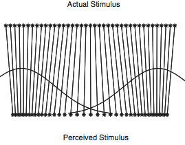
Example: Categorical Perception of Speech Sounds

(This example is adapted from: Feldman, N. H., Griffiths, T. L., and Morgan, J. L. (2009). The influence of categories on perception: Explaining the perceptual magnet effect as optimal statistical inference. Psychological Review, 116(4):752–782.)

Human perception is often skewed by our expectations. A common example of this is called categorical perception – when we perceive objects as being more similar to the category prototype than they really are. In phonology this is been particularly important and is called the perceptual magnet effect: Hearers regularize a speech sound into the category that they think it corresponds to. Of course this category isn’t known a priori, so a hearer must be doing a simultaneous inference of what category the speech sound corresponded to, and what the sound must have been. In the below code we model this as a mixture model over the latent categories of sounds, combined with a noisy observation process.

(define (count-by start end increment)
  (if (> start end)
      '()
      (pair start (count-by (+ start increment) end increment))))

(define (expectation l)
  (/ (apply + l) (length l)))

(define prototype-1 8.0)
(define prototype-2 10.0)

(define (compute-pair-distance stimulus-1 stimulus-2)
  (expectation
   (mh-query
    2000 10

    (define (vowel-1) (gaussian prototype-1 0.5))
    (define (vowel-2) (gaussian prototype-2 0.5))

    (define (noise-process target)
      (gaussian target 0.2))

    (define (sample-target)
      (if (flip)
          (vowel-1)
          (vowel-2)))

    (define target-1 (sample-target))
    (define target-2 (sample-target))

    (define obs-1 (noise-process target-1))
    (define obs-2 (noise-process target-2))

    (abs (- target-1 target-2))

    ;;Condition on the targets being equal to the stimuli through a gaussian noise process
    (and 
      (= stimulus-1 (gaussian target-1 0.2))
      (= stimulus-2 (gaussian target-2 0.2))))))

(define (compute-perceptual-pairs list)
  (if (< (length list) 2)
      '()
      (pair (compute-pair-distance (first list) (second list)) (compute-perceptual-pairs (rest list)))))

(define (compute-stimuli-pairs list)
  (if (< (length list) 2)
      '()
      (pair (abs (- (first list) (second list))) (compute-stimuli-pairs (rest list)))))

(define stimuli (count-by prototype-1 prototype-2 0.1))

(define stimulus-distances (compute-stimuli-pairs stimuli))
(define perceptual-distances (compute-perceptual-pairs stimuli))

(scatter (map pair (iota (- (length stimuli) 1))
              stimulus-distances)
         "Stimulus Distances")

(scatter (map pair (iota (- (length stimuli) 1))
              perceptual-distances)
         "Perceptual Distances")

Notice that the perceived distances between input sounds are skewed relative to the actual acoustic distances – that is they are attracted towards the category centers.

Unknown Numbers of Categories

The models above describe how a learner can simultaneously learn which category each object belongs to, the typical properties of objects in that category, and even global parameters about kinds of objects in general. However, it suffers from a serious flaw: the number of categories was fixed. This is as if a learner, after finding out there are cats, dogs, and mice, must force an elephant into one of these categories, for want of more categories to work with.

The simplest way to address this problem, which we call unbounded models, is be to simply place uncertainty on the number of categories in the form of a hierarchical prior. Let’s warm up with a simple example of this: inferring whether one or two coins were responsible for a set of outcomes (i.e. imagine a friend is shouting each outcome from the next room–“heads, heads, tails…”–is she using a fair coin, or two biased coins?).

(define actual-obs (list true true true true false false false false))

(define samples
 (mh-query
   200 100

   (define coins (if (flip) '(c1) '(c1 c2)))

   (define coin->weight (mem (lambda (c) (uniform 0 1))))

   (define (observe values)
     (map (lambda (v)
       (condition (equal? (flip (coin->weight (uniform-draw coins))) v))) values))

   (length coins)

   (observe actual-obs)))

(hist samples "number of coins")
'done

How does the inferred number of coins change as the amount of data grows? Why?

We could extend this model by allowing it to infer that there are more than two coins. However, no evidence requires us to posit three or more coins (we can always explain the data as “a heads coin and a tails coin”). Instead, let us apply the same idea to the marbles examples above:

(define colors '(blue green red))

(define samples
  (mh-query
   200 100

   (define phi (dirichlet '(1 1 1)))
   (define alpha 0.1)
   (define prototype (map (lambda (w) (* alpha w)) phi))

   (define bag->prototype (mem (lambda (bag) (dirichlet prototype))))

   ;;unknown number of categories (created with placeholder names):
   (define num-bags (+ 1 (poisson 1.0)))

   (define bags (repeat num-bags gensym))

   (define (observe marbles)
     (map (lambda (m) (condition (equal? (multinomial colors (bag->prototype (uniform-draw bags))) m))) marbles))

   ;;how many bags are there?
   num-bags

   (observe '(red red blue blue red blue))))

(hist samples "how many bags?")
'done

Vary the amount of evidence and see how the inferred number of bags changes.

For the prior on num-bags we used the Poisson distribution which is a distribution on non-negative integers. It is convenient, though implies strong prior knowledge (perhaps too strong for this example). We have created gensym functions using make-gensym; a gensym function returns a fresh symbol every time it is called. It can be used to generate an unbounded set of labels for things like classes, categories and mixture components. Each evaluation of gensym results in a unique (although cryptic) symbol:

(list (gensym) (gensym) (gensym))

Importantly, these symbols can be used as identifiers, because two different calls to gensym will never be equal:

(equal? (gensym) (gensym))

For clarity, you can use the make-gensym to create a gensym function with a custom prefix:

(define my-gensym (make-gensym "foo"))
(list (my-gensym) (my-gensym) (my-gensym))

Unbounded models give a straightforward way to represent uncertainty over the number of categories in the world. However, inference in these models often presents difficulties. In the next section we describe another method for allowing an unknown number of things: In an unbounded model, there are a finite number of categories whose number is drawn from an unbounded prior distribution, such as the Poisson prior that we just examined. In an ‘infinite model’ we construct distributions assuming a truly infinite numbers of objects.